Circuits variationnels quantiques et réseaux de neurones quantiques
Dans cette leçon, nous implémentons plusieurs circuits quantiques variationnels pour une tâche de classification de données, appelés classificateurs quantiques variationnels (VQC). À un moment donné, il était courant de qualifier un sous-ensemble des VQC de réseaux de neurones quantiques (RNQ) par analogie avec les réseaux de neurones classiques. En effet, il existe des cas où les structures empruntées aux réseaux de neurones classiques, comme les couches de convolution, jouent un rôle important dans les VQC. Dans ces cas où l'analogie est forte, les RNQ peuvent être une description utile. Cependant, les circuits quantiques paramétrés ne doivent pas nécessairement suivre la structure générale d'un réseau de neurones ; par exemple, tous les données n'ont pas besoin d'être chargées dans la première couche (couche d'entrée) : nous pouvons charger certaines données dans la première couche, appliquer certaines portes, puis charger d'autres données (un processus appelé « ré-importation » de données). Par conséquent, nous devrions considérer les RNQ comme un sous-ensemble des circuits quantiques paramétrés, et nous ne devrions pas limiter notre exploration des circuits quantiques utiles par l'analogie avec les réseaux de neurones classiques.
L'ensemble de données abordé dans cette leçon est composé d'images contenant des rayures horizontales et verticales, et notre objectif est de classer les images invisibles dans l'une des deux catégories selon l'orientation de la ligne. Nous accomplissons ceci avec un VQC. En chemin, nous explorerons les façons d'améliorer et de mettre à l'échelle le calcul. L'ensemble de données ici est exceptionnellement facile à classer classiquement. Il a été choisi pour sa simplicité afin que nous puissions nous concentrer sur la partie quantique de ce problème, et voir comment un attribut de l'ensemble de données pourrait se traduire par une partie d'un circuit quantique. Il n'est pas raisonnable de s'attendre à une accélération quantique pour des cas aussi simples où les algorithmes classiques sont si efficaces.
À la fin de cette leçon, tu devrais être capable de :
- Charger des données d'une image dans un circuit quantique
- Construire un ansatz pour un VQC (ou RNQ), et l'adapter à ton problème
- Entraîner ton VQC/RNQ et l'utiliser pour faire des prédictions précises sur les données de test
- Mettre à l'échelle le problème et reconnaître les limites des ordinateurs quantiques actuels
Génération de données
Nous commencerons par construire les données. Les ensembles de données ne sont souvent pas générés explicitement dans le cadre des motifs Qiskit. Cependant, le type et la préparation des données sont essentiels pour appliquer avec succès l'informatique quantique à l'apprentissage automatique. Le code ci-dessous définit un ensemble de données d'images avec des dimensions de pixels définies. Une rangée ou colonne complète de l'image se voit attribuer la valeur , et les pixels restants se voient attribuer des valeurs aléatoires dans l'intervalle . Les valeurs aléatoires constituent du bruit dans nos données. Examine le code pour t'assurer que tu comprends comment les images sont générées. Plus tard, nous augmenterons la taille des images.
# Added by doQumentation — required packages for this notebook
!pip install -q matplotlib numpy qiskit qiskit-ibm-runtime scipy scikit-learn
# This code defines the images to be classified:

import numpy as np

# Total number of "pixels"/qubits
size = 8
# One dimension of the image (called vertical, but it doesn't matter). Must be a divisor of `size`
vert_size = 2
# The length of the line to be detected (yellow). Must be less than or equal to the smallest
# dimension of the image (`<=min(vert_size,size/vert_size)`
line_size = 2

def generate_dataset(num_images):
    images = []
    labels = []
    hor_array = np.zeros((size - (line_size - 1) * vert_size, size))
    ver_array = np.zeros((round(size / vert_size) * (vert_size - line_size + 1), size))

    j = 0
    for i in range(0, size - 1):
        if i % (size / vert_size) <= (size / vert_size) - line_size:
            for p in range(0, line_size):
                hor_array[j][i + p] = np.pi / 2
            j += 1

    # Make two adjacent entries pi/2, then move down to the next row. Careful to avoid the "pixels"
    # at size/vert_size - linesize, because we want to fold this list into a grid.

    j = 0
    for i in range(0, round(size / vert_size) * (vert_size - line_size + 1)):
        for p in range(0, line_size):
            ver_array[j][i + p * round(size / vert_size)] = np.pi / 2
        j += 1

    # Make entries pi/2, spaced by the length/rows, so that when folded,
    # the entries appear on top of each other.

    for n in range(num_images):
        rng = np.random.randint(0, 2)
        if rng == 0:
            labels.append(-1)
            random_image = np.random.randint(0, len(hor_array))
            images.append(np.array(hor_array[random_image]))

        elif rng == 1:
            labels.append(1)
            random_image = np.random.randint(0, len(ver_array))
            images.append(np.array(ver_array[random_image]))
            # Randomly select 0 or 1 for a horizontal or vertical array, assign the corresponding
            # label.

        # Create noise
        for i in range(size):
            if images[-1][i] == 0:
                images[-1][i] = np.random.rand() * np.pi / 4
    return images, labels

hor_size = round(size / vert_size)
Note que le code ci-dessus a également généré des étiquettes indiquant si les images contiennent une ligne verticale (+1) ou horizontale (-1). Nous allons maintenant utiliser sklearn pour diviser un ensemble de données de 100 images en un ensemble d'entraînement et un ensemble de test (ainsi que leurs étiquettes correspondantes). Ici, nous utilisons de l'ensemble de données pour l'entraînement, en réservant les restants pour les tests.
from sklearn.model_selection import train_test_split

np.random.seed(42)
images, labels = generate_dataset(200)

train_images, test_images, train_labels, test_labels = train_test_split(
    images, labels, test_size=0.3, random_state=246
)
Traçons quelques éléments de notre ensemble de données pour voir à quoi ressemblent ces lignes :
import matplotlib.pyplot as plt

# Make subplot titles so we can identify categories
titles = []
for i in range(8):
    title = "category: " + str(train_labels[i])
    titles.append(title)

# Generate a figure with nested images using subplots.
fig, ax = plt.subplots(4, 2, figsize=(10, 6), subplot_kw={"xticks": [], "yticks": []})

for i in range(8):
    ax[i // 2, i % 2].imshow(
        train_images[i].reshape(vert_size, hor_size),
        aspect="equal",
    )
    ax[i // 2, i % 2].set_title(titles[i])
plt.subplots_adjust(wspace=0.1, hspace=0.3)

Chacune de ces images est toujours associée à son étiquette dans train_labels sous forme de liste simple :
print(train_labels[:8])
[1, 1, 1, 1, -1, 1, 1, 1]
Classificateur quantique variationnel : une première tentative
Étape 1 des motifs Qiskit : Mapper le problème à un circuit quantique
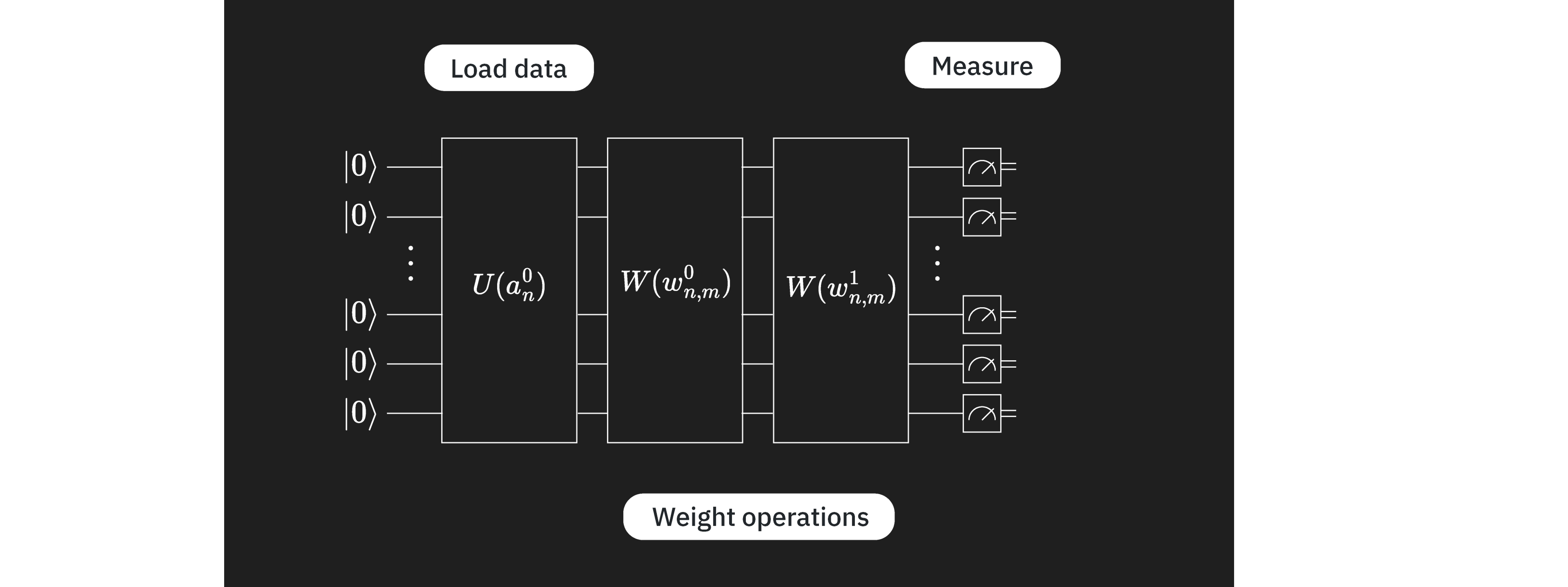
L'objectif est de trouver une fonction avec des paramètres qui mappe un vecteur de données / image à la catégorie correcte : . Ceci sera réalisé en utilisant un VQC avec peu de couches pouvant être identifiées par leurs objectifs distincts :
Ici, est le circuit d'encodage, pour lequel nous avons de nombreuses options comme on l'a vu dans les leçons précédentes. est un bloc de circuit variationnel ou entraînable, et est l'ensemble des paramètres à entraîner. Ces paramètres seront variés par des algorithmes d'optimisation classiques pour trouver l'ensemble de paramètres qui donne la meilleure classification des images par le circuit quantique. Ce circuit variationnel est parfois appelé l'« ansatz ». Enfin, est un observable qui sera estimé en utilisant la primitive Estimator. Il n'y a aucune contrainte obligeant les couches à venir dans cet ordre, ou même à être complètement séparées. On pourrait avoir plusieurs couches variationnelles et/ou d'encodage dans n'importe quel ordre qui est techniquement motivé.
Nous commençons par choisir une carte de caractéristiques pour encoder nos données. Nous utiliserons le z_feature_map, car il maintient les profondeurs de circuits basses par rapport à d'autres encodages de caractéristiques.
from qiskit.circuit.library import z_feature_map

# One qubit per data feature
num_qubits = len(train_images[0])

# Data encoding
# Note that qiskit orders parameters alphabetically. We assign the parameter prefix "a" to ensure
# our data encoding goes to the first part of the circuit, the feature mapping.
feature_map = z_feature_map(num_qubits, parameter_prefix="a")
Nous devons maintenant décider d'un ansatz à entraîner. Il y a de nombreuses considérations lors du choix d'un ansatz. Une description complète dépasse le cadre de cette introduction ; ici, nous soulignons simplement quelques catégories de considérations.
- Matériel : Tous les ordinateurs quantiques modernes sont plus sujets aux erreurs et plus susceptibles au bruit que leurs homologues classiques. Utiliser un ansatz excessivement profond (surtout en profondeur de portes à deux qubits transpilée) ne donnera pas de bons résultats. Un problème connexe est que les ordinateurs quantiques ont une certaine disposition de qubits, ce qui signifie que certains qubits physiques sont adjacents sur l'ordinateur quantique, tandis que d'autres peuvent être très éloignés les uns des autres. L'intrication de qubits adjacents n'augmente pas trop la profondeur, mais l'intrication de qubits très distants peut augmenter la profondeur substantiellement, car nous devons insérer des portes d'échange pour déplacer les informations vers des qubits qui sont adjacents pour pouvoir les entrelacer.
- Le problème : Chaque fois que tu as des informations sur ton problème qui pourraient guider ton ansatz, utilise-les. Par exemple, les données de cette leçon sont composées d'images de lignes horizontales et verticales. On pourrait considérer quelle corrélation entre les valeurs/couleurs adjacentes identifie une image d'une ligne horizontale ou verticale. Quels attributs d'un ansatz correspondraient à cette corrélation entre pixels adjacents ? Nous revisiterons ce point plus techniquement plus tard dans cette leçon. Mais pour l'instant, disons simplement que l'inclusion de l'intrication et des portes CNOT entre les qubits correspondant aux pixels adjacents semble une bonne idée. Dans le tableau plus large, considère si le problème est vraiment mieux résolu en utilisant un circuit quantique, ou si des algorithmes classiques pourraient faire aussi bien.
- Nombre de paramètres : Chaque porte quantique indépendamment paramétrée du circuit augmente l'espace à optimiser classiquement, ce qui entraîne une convergence plus lente. Mais à mesure que les problèmes augmentent en taille, tu pourrais rencontrer des plateaux stériles. Ce terme fait référence à un phénomène où le paysage d'optimisation d'un algorithme quantique variationnel devient exponentiellement plat et sans caractéristiques à mesure que la taille du problème augmente. Cela provoque des gradients qui disparaissent, rendant difficile l'entraînement efficace de l'algorithme[1]. Les plateaux stériles sont pertinents pour les algorithmes quantiques variationnels comme les VQC/RNQ. Il convient de noter que l'augmentation du nombre de paramètres n'est pas la seule considération pour éviter les plateaux stériles ; d'autres considérations incluent les fonctions de coût globales et l'initialisation aléatoire des paramètres.
Dans cette leçon, nous verrons quelques exemples simples de bonnes pratiques dans la construction d'ansatz. Essayons d'abord l'ansatz ci-dessous. Nous y reviendrons plus tard.
# Import the necessary packages
from qiskit import QuantumCircuit
from qiskit.circuit import ParameterVector

# Initialize the circuit using the same number of qubits as the image has pixels
qnn_circuit = QuantumCircuit(size)

# We choose to have two variational parameters for each qubit.
params = ParameterVector("θ", length=2 * size)

# A first variational layer:
for i in range(size):
    qnn_circuit.ry(params[i], i)

# Here is a list of qubit pairs between which we want CNOT gates.
# The choice of these is not yet obvious.
qnn_cnot_list = [[0, 1], [1, 2], [2, 3]]

for i in range(len(qnn_cnot_list)):
    qnn_circuit.cx(qnn_cnot_list[i][0], qnn_cnot_list[i][1])

# The second variational layer:
for i in range(size):
    qnn_circuit.rx(params[size + i], i)

# Check the circuit depth, and the two-qubit gate depth
print(qnn_circuit.decompose().depth())
print(
    f"2+ qubit depth: {qnn_circuit.decompose().depth(lambda instr: len(instr.qubits) > 1)}"
)

# Draw the circuit
qnn_circuit.draw("mpl")
5
2+ qubit depth: 3
┌──────────┐             ┌──────────┐
q_0: ┤ Ry(θ[0]) ├──────■──────┤ Rx(θ[8]) ├─────────────────────────
     ├──────────┤    ┌─┴─┐    └──────────┘┌──────────┐
q_1: ┤ Ry(θ[1]) ├────┤ X ├─────────■──────┤ Rx(θ[9]) ├─────────────
     ├──────────┤    └───┘       ┌─┴─┐    └──────────┘┌───────────┐
q_2: ┤ Ry(θ[2]) ├────────────────┤ X ├─────────■──────┤ Rx(θ[10]) ├
     ├──────────┤                └───┘       ┌─┴─┐    ├───────────┤
q_3: ┤ Ry(θ[3]) ├────────────────────────────┤ X ├────┤ Rx(θ[11]) ├
     ├──────────┤┌───────────┐               └───┘    └───────────┘
q_4: ┤ Ry(θ[4]) ├┤ Rx(θ[12]) ├─────────────────────────────────────
     ├──────────┤├───────────┤
q_5: ┤ Ry(θ[5]) ├┤ Rx(θ[13]) ├─────────────────────────────────────
     ├──────────┤├───────────┤
q_6: ┤ Ry(θ[6]) ├┤ Rx(θ[14]) ├─────────────────────────────────────
     ├──────────┤├───────────┤
q_7: ┤ Ry(θ[7]) ├┤ Rx(θ[15]) ├─────────────────────────────────────
     └──────────┘└───────────┘
Avec l'encodage des données et le circuit variationnel préparés, nous pouvons les combiner pour former notre ansatz complet. Dans ce cas, les composants de notre circuit quantique sont assez analogues à ceux des réseaux de neurones, avec étant le plus similaire à la couche qui charge les valeurs d'entrée de l'image, et étant comme la couche des « poids » variables. Puisque cette analogie tient dans ce cas, nous adoptons « rnn » dans certaines de nos conventions de nommage ; mais cette analogie ne doit pas limiter ton exploration des VQC.
# QNN ansatz
ansatz = qnn_circuit

# Combine the feature map with the ansatz
full_circuit = QuantumCircuit(num_qubits)
full_circuit.compose(feature_map, range(num_qubits), inplace=True)
full_circuit.compose(ansatz, range(num_qubits), inplace=True)

# Display the circuit
full_circuit.decompose().draw("mpl", style="clifford", fold=-1)

Nous devons maintenant définir un observable, pour pouvoir l'utiliser dans notre fonction de coût. Nous obtiendrons une valeur attendue pour cet observable en utilisant Estimator. Si tu as sélectionné un ansatz bon et motivé par le problème, alors chaque qubit contiendra des informations pertinentes pour la classification. On peut ajouter des couches pour combiner les informations sur moins de qubits (appelée une couche de convolution), de sorte que les mesures ne soient nécessaires que sur un sous-ensemble des qubits du circuit (comme dans les réseaux de neurones convolutifs). Ou tu peux mesurer un attribut de chaque qubit. Ici, nous opterons pour ce dernier, donc nous incluons un opérateur Z pour chaque qubit. Il n'y a rien d'unique à choisir , mais c'est bien motivé :
- C'est une tâche de classification binaire, et une mesure de peut donner deux résultats possibles.
- Les valeurs propres de () sont raisonnablement bien séparées, et donnent un résultat estimateur dans l'intervalle [-1, +1], où 0 peut simplement être utilisé comme valeur de coupure.
- Il est simple de mesurer dans la base de Pauli Z sans surcharge supplémentaire de porte.
Ainsi, Z est un choix très naturel.
from qiskit.quantum_info import SparsePauliOp

observable = SparsePauliOp.from_list([("Z" * (num_qubits), 1)])
Nous avons notre circuit quantique et l'observable que nous voulons estimer. Maintenant, nous avons besoin de quelques choses pour exécuter et optimiser ce circuit. D'abord, nous avons besoin d'une fonction pour exécuter une passe avant. Note que la fonction ci-dessous prend input_params et weight_params séparément. Le premier est l'ensemble des paramètres statiques décrivant les données dans une image, et le second est l'ensemble des paramètres variables à optimiser.
from qiskit.primitives import BaseEstimatorV2
from qiskit.quantum_info.operators.base_operator import BaseOperator

def forward(
    circuit: QuantumCircuit,
    input_params: np.ndarray,
    weight_params: np.ndarray,
    estimator: BaseEstimatorV2,
    observable: BaseOperator,
) -> np.ndarray:
    """
    Forward pass of the neural network.

    Args:
        circuit: circuit consisting of data loader gates and the neural network ansatz.
        input_params: data encoding parameters.
        weight_params: neural network ansatz parameters.
        estimator: EstimatorV2 primitive.
        observable: a single observable to compute the expectation over.

    Returns:
        expectation_values: an array (for one observable) or a matrix (for a sequence of observables) of expectation values.
        Rows correspond to observables and columns to data samples.
    """
    num_samples = input_params.shape[0]
    weights = np.broadcast_to(weight_params, (num_samples, len(weight_params)))
    params = np.concatenate((input_params, weights), axis=1)
    pub = (circuit, observable, params)
    job = estimator.run([pub])
    result = job.result()[0]
    expectation_values = result.data.evs

    return expectation_values
Fonction de perte
Ensuite, nous avons besoin d'une fonction de perte pour calculer la différence entre les valeurs prédites et calculées des étiquettes. La fonction prendra les étiquettes prédites par l'algorithme et les étiquettes correctes, et retournera la différence quadratique moyenne. Il y a de nombreuses fonctions de perte différentes. Ici, MSE est un exemple que nous avons choisi.
def mse_loss(predict: np.ndarray, target: np.ndarray) -> np.ndarray:
    """
    Mean squared error (MSE).

    prediction: predictions from the forward pass of neural network.
    target: true labels.

    output: MSE loss.
    """
    if len(predict.shape) <= 1:
        return ((predict - target) ** 2).mean()
    else:
        raise AssertionError("input should be 1d-array")
Définissons également une fonction de perte légèrement différente qui est une fonction des paramètres variables (poids), à utiliser par l'optimiseur classique. Cette fonction ne prend que les paramètres de l'ansatz en entrée ; les autres variables pour la passe avant et la perte sont définies comme paramètres globaux. L'optimiseur entraînera le modèle en échantillonnant différents poids et en essayant de réduire la sortie de la fonction de coût/perte.
def mse_loss_weights(weight_params: np.ndarray) -> np.ndarray:
    """
    Cost function for the optimizer to update the ansatz parameters.

    weight_params: ansatz parameters to be updated by the optimizer.

    output: MSE loss.
    """
    predictions = forward(
        circuit=circuit,
        input_params=input_params,
        weight_params=weight_params,
        estimator=estimator,
        observable=observable,
    )

    cost = mse_loss(predict=predictions, target=target)
    objective_func_vals.append(cost)

    global iter
    if iter % 50 == 0:
        print(f"Iter: {iter}, loss: {cost}")
    iter += 1

    return cost
Ci-dessus, nous avons mentionné l'utilisation d'un optimiseur classique. Quand nous en arriverons à rechercher parmi les poids pour minimiser la fonction de coût, nous utiliserons l'optimiseur COBYLA :
from scipy.optimize import minimize
Nous allons définir quelques variables globales initiales pour la fonction de coût.
# Globals
circuit = full_circuit
observables = observable
# input_params = train_images_batch
# target = train_labels_batch
objective_func_vals = []
iter = 0
Étape 2 des motifs Qiskit : Optimiser le problème pour l'exécution quantique
Nous commençons par sélectionner un backend pour l'exécution. Dans ce cas, nous utiliserons le backend le moins occupé.
from qiskit_ibm_runtime import QiskitRuntimeService

service = QiskitRuntimeService()
backend = service.least_busy(operational=True, simulator=False)
print(backend.name)
ibm_brisbane
Ici, nous optimisons le circuit pour fonctionner sur un backend réel en spécifiant le optimization_level et en ajoutant le découplage dynamique. Le code ci-dessous génère un gestionnaire de passe en utilisant les gestionnaires de passe prédéfinis de qiskit.transpiler.
from qiskit.circuit.library import XGate
from qiskit.transpiler import PassManager
from qiskit.transpiler.passes import (
    ALAPScheduleAnalysis,
    ConstrainedReschedule,
    PadDynamicalDecoupling,
)
from qiskit.transpiler.preset_passmanagers import generate_preset_pass_manager

target = backend.target

pm = generate_preset_pass_manager(target=target, optimization_level=3)
pm.scheduling = PassManager(
    [
        ALAPScheduleAnalysis(target=target),
        ConstrainedReschedule(
            acquire_alignment=target.acquire_alignment,
            pulse_alignment=target.pulse_alignment,
            target=target,
        ),
        PadDynamicalDecoupling(
            target=target,
            dd_sequence=[XGate(), XGate()],
            pulse_alignment=target.pulse_alignment,
        ),
    ]
)
Maintenant nous appliquons le gestionnaire de passe au circuit. Les changements de disposition qui en résultent doivent également être appliqués à l'observable. Pour les circuits très grands, les heuristiques utilisées dans l'optimisation des circuits peuvent ne pas toujours donner le circuit le plus efficace et le plus superficiel. Dans ces cas, il est judicieux d'exécuter ces gestionnaires de passe plusieurs fois et d'utiliser le meilleur circuit. Nous verrons ceci plus tard quand nous augmenterons notre calcul.
circuit_ibm = pm.run(full_circuit)
observable_ibm = observable.apply_layout(circuit_ibm.layout)
Étape 3 des motifs Qiskit : Exécuter en utilisant les primitives Qiskit
Boucler sur l'ensemble de données en lots et en époques
Nous commençons par implémenter l'algorithme complet en utilisant un simulateur pour le débogage préliminaire et pour les estimations d'erreur. Nous pouvons maintenant parcourir tout l'ensemble de données en lots sur le nombre d'époques souhaité pour entraîner notre réseau de neurones quantiques.
from qiskit.primitives import StatevectorEstimator as Estimator

batch_size = 140
num_epochs = 1
num_samples = len(train_images)

# Globals
circuit = full_circuit
estimator = Estimator()  # simulator for debugging
observables = observable
objective_func_vals = []
iter = 0

# Random initial weights for the ansatz
np.random.seed(42)
weight_params = np.random.rand(len(ansatz.parameters)) * 2 * np.pi

for epoch in range(num_epochs):
    for i in range((num_samples - 1) // batch_size + 1):
        print(f"Epoch: {epoch}, batch: {i}")
        start_i = i * batch_size
        end_i = start_i + batch_size
        train_images_batch = np.array(train_images[start_i:end_i])
        train_labels_batch = np.array(train_labels[start_i:end_i])
        input_params = train_images_batch
        target = train_labels_batch
        iter = 0
        res = minimize(
            mse_loss_weights, weight_params, method="COBYLA", options={"maxiter": 100}
        )
        weight_params = res["x"]
Epoch: 0, batch: 0
Iter: 0, loss: 1.0002309063537163
Iter: 50, loss: 0.9434121445008878
Étape 4 des motifs Qiskit : Post-traiter, retourner le résultat au format classique
Test et précision
Nous interprétons maintenant les résultats de l'entraînement. Nous testons d'abord la précision de l'entraînement sur l'ensemble d'entraînement.
import copy
from sklearn.metrics import accuracy_score
from qiskit.primitives import StatevectorEstimator as Estimator  # simulator
# from qiskit_ibm_runtime import EstimatorV2 as Estimator  # real quantum computer

estimator = Estimator()
# estimator = Estimator(backend=backend)

pred_train = forward(circuit, np.array(train_images), res["x"], estimator, observable)
# pred_train = forward(circuit_ibm, np.array(train_images), res['x'], estimator, observable_ibm)

print(pred_train)

pred_train_labels = copy.deepcopy(pred_train)
pred_train_labels[pred_train_labels >= 0] = 1
pred_train_labels[pred_train_labels < 0] = -1
print(pred_train_labels)
print(train_labels)

accuracy = accuracy_score(train_labels, pred_train_labels)
print(f"Train accuracy: {accuracy * 100}%")
[-2.27688499e-02 -1.46227204e-02 -1.73927452e-02  9.93331786e-02
 -4.85553548e-01  1.43558565e-01  8.34567054e-02 -1.40133992e-02
  1.52169596e-01 -1.95082515e-01  8.24373578e-03 -9.90696638e-02
 -3.54268344e-02 -4.77017954e-01  1.38713848e-02 -2.99706215e-01
 -5.78378029e-02  3.25528779e-02 -4.11354239e-02 -1.06483708e-01
  1.53095800e-01  2.90110884e-02  1.25745450e-02  6.46323079e-02
 -1.53538943e-01 -1.57694952e-02 -1.67800067e-02 -1.99820822e-01
  1.70360075e-01  7.86148038e-03 -2.33373818e-02  6.64233020e-02
 -1.14895445e-01 -1.11296215e-01  1.15120303e-01 -2.94096140e-01
 -1.00531392e-03 -1.69209726e-01 -1.26120885e-01  3.26298176e-02
 -1.33517383e-02 -5.86983444e-02 -4.32341361e-01 -4.36509551e-01
 -4.17940102e-02  1.76935235e-03  8.14479984e-03  1.86985655e-01
 -2.75525019e-01 -1.63229907e-03 -1.08571055e-01 -7.37452387e-04
 -6.44440657e-02  6.72812834e-04  2.16785530e-03  1.41381850e-01
 -9.82570410e-02  4.35973325e-01 -7.62261965e-02 -1.86193980e-01
 -1.56971183e-02 -4.02757541e-01 -1.53869367e-01  2.29262129e-02
 -7.02788246e-03  3.65719683e-02  4.68232163e-01  2.36434668e-02
 -2.59520939e-02  3.70550137e-01 -1.19630110e-01 -5.79555318e-02
  2.09554455e-01  5.04689780e-02  7.39494314e-02 -1.77647326e-02
 -1.45407207e-01 -9.54908878e-02  7.56029640e-02 -2.74049696e-02
  3.34885873e-01  1.58546171e-03  1.09339091e-01 -8.84693274e-02
 -2.36450457e-02  1.41892239e-01 -2.34453218e-01 -7.50717757e-02
 -1.13281310e-01 -1.66649414e-01 -3.17224197e-01 -6.38220597e-02
  3.28916563e-02  3.04739203e-02  2.67720196e-02 -1.16485785e-01
 -3.08115732e-02 -2.95372010e-02 -7.54669023e-02  6.20013872e-02
 -3.85258710e-01 -1.16456443e-01 -7.38548075e-02 -3.20558243e-02
 -4.22284741e-02  1.01285659e-01 -1.76949246e-01 -2.02767491e-01
 -1.12407344e-01 -3.81408267e-02 -4.33345231e-01 -9.24507501e-02
 -4.21765393e-02 -6.06533771e-02 -2.22257783e-01 -1.17312535e-01
 -6.74132262e-02 -2.76206274e-01 -9.13971800e-02 -2.27653991e-01
  1.66358563e-01  2.17230774e-04  5.76426304e-02 -2.82079169e-02
 -1.15482051e-01 -3.46716009e-01 -3.21448755e-01 -5.20041405e-02
 -2.16833625e-01 -1.06154654e-02 -7.74854811e-02 -3.28257935e-01
 -7.83242410e-02  1.65547682e-01 -2.55294862e-01 -8.89085025e-02
  4.47581491e-01  1.92351832e-02  2.74083885e-02 -3.61304571e-01]
[-1. -1. -1.  1. -1.  1.  1. -1.  1. -1.  1. -1. -1. -1.  1. -1. -1.  1.
 -1. -1.  1.  1.  1.  1. -1. -1. -1. -1.  1.  1. -1.  1. -1. -1.  1. -1.
 -1. -1. -1.  1. -1. -1. -1. -1. -1.  1.  1.  1. -1. -1. -1. -1. -1.  1.
  1.  1. -1.  1. -1. -1. -1. -1. -1.  1. -1.  1.  1.  1. -1.  1. -1. -1.
  1.  1.  1. -1. -1. -1.  1. -1.  1.  1.  1. -1. -1.  1. -1. -1. -1. -1.
 -1. -1.  1.  1.  1. -1. -1. -1. -1.  1. -1. -1. -1. -1. -1.  1. -1. -1.
 -1. -1. -1. -1. -1. -1. -1. -1. -1. -1. -1. -1.  1.  1.  1. -1. -1. -1.
 -1. -1. -1. -1. -1. -1. -1.  1. -1. -1.  1.  1.  1. -1.]
[1, 1, 1, 1, -1, 1, 1, 1, -1, 1, 1, 1, -1, -1, -1, -1, -1, -1, -1, -1, 1, -1, 1, 1, -1, 1, 1, 1, 1, -1, 1, 1, -1, 1, 1, -1, 1, 1, -1, -1, -1, 1, -1, -1, 1, -1, 1, 1, -1, 1, -1, 1, 1, -1, 1, 1, 1, 1, -1, -1, -1, -1, 1, -1, 1, 1, 1, -1, -1, 1, 1, -1, 1, 1, -1, -1, 1, -1, 1, 1, 1, 1, 1, -1, -1, 1, -1, -1, -1, -1, -1, 1, 1, -1, -1, 1, -1, -1, 1, 1, -1, 1, -1, 1, 1, 1, 1, 1, -1, -1, -1, 1, -1, -1, -1, 1, -1, -1, 1, -1, 1, -1, 1, 1, -1, -1, -1, 1, 1, 1, -1, -1, -1, 1, -1, 1, 1, -1, -1, -1]
Train accuracy: 60.0%
pred_test = forward(circuit, np.array(test_images), res["x"], estimator, observable)
# pred_test = forward(circuit_ibm, np.array(test_images), res['x'], estimator, observable_ibm)

print(pred_test)

pred_test_labels = copy.deepcopy(pred_test)
pred_test_labels[pred_test_labels >= 0] = 1
pred_test_labels[pred_test_labels < 0] = -1
print(pred_test_labels)
print(test_labels)

accuracy = accuracy_score(test_labels, pred_test_labels)
print(f"Test accuracy: {accuracy * 100}%")
[-2.77978120e-01 -2.62194862e-01  4.59636095e-02 -8.09344165e-02
 -2.97362966e-01  9.22947242e-02  2.06693174e-01  3.31629460e-02
  1.10971762e-03 -2.14602152e-01 -1.62671993e-01 -6.07179155e-04
 -1.59948633e-01 -8.55722523e-02 -1.13057027e-01 -3.00187433e-01
 -2.92832827e-01  7.38580629e-02 -6.03706270e-02 -8.57643552e-02
 -1.52402062e-02 -3.57505447e-01 -3.54890597e-02  1.36534749e-01
 -1.54688180e-01 -2.93714726e-01  1.89548513e-02 -6.15715564e-02
  1.11042670e-01 -2.22861100e-02 -3.84230105e-02  1.67351034e-01
 -8.38766333e-02  2.56348613e-01 -1.10653111e-01 -1.18989476e-01
 -6.75723266e-05 -6.88580547e-02  1.02431393e-02 -2.42125353e-01
 -1.09142367e-01 -1.22540757e-01 -1.63735850e-01  3.93334838e-01
  2.36705685e-01 -2.34259814e-02 -3.91877756e-02 -1.95106746e-01
  1.86707523e-01  4.74775215e-02 -4.24907432e-02 -2.06453265e-01
  4.09184710e-02 -3.54762080e-02 -9.47513112e-02  2.97270112e-01
 -2.99708696e-02  9.93941064e-03 -1.26760302e-01 -1.36183355e-01]
[-1. -1.  1. -1. -1.  1.  1.  1.  1. -1. -1. -1. -1. -1. -1. -1. -1.  1.
 -1. -1. -1. -1. -1.  1. -1. -1.  1. -1.  1. -1. -1.  1. -1.  1. -1. -1.
 -1. -1.  1. -1. -1. -1. -1.  1.  1. -1. -1. -1.  1.  1. -1. -1.  1. -1.
 -1.  1. -1.  1. -1. -1.]
[-1, -1, 1, 1, -1, -1, 1, -1, 1, -1, 1, 1, 1, 1, -1, 1, -1, 1, 1, 1, 1, -1, -1, 1, 1, -1, 1, 1, 1, -1, 1, -1, -1, 1, 1, 1, -1, 1, 1, -1, -1, -1, 1, 1, 1, -1, 1, 1, 1, 1, -1, -1, 1, 1, 1, 1, 1, 1, -1, -1]
Test accuracy: 60.0%
Le modèle ne classe pas bien ces données. Nous devrions nous demander pourquoi c'est le cas et, en particulier, nous devrions vérifier :
- Avons-nous arrêté l'entraînement trop tôt ? Plus d'étapes d'optimisation étaient-elles nécessaires ?
- Avons-nous construit un mauvais ansatz ? Cela pourrait signifier beaucoup de choses. Quand nous travaillons sur de vrais ordinateurs quantiques, la profondeur du circuit sera une considération majeure. Le nombre de paramètres est également potentiellement important, tout comme l'intrication entre les qubits.
- Combinant les deux ci-dessus, avons-nous construit un ansatz avec trop de paramètres pour être entraînable ?
Nous pouvons commencer par vérifier la convergence de l'optimisation :
obj_func_vals_first = objective_func_vals
# import matplotlib.pyplot as plt

plt.figure(figsize=(12, 6))
plt.plot(obj_func_vals_first, label="first ansatz")
plt.xlabel("iteration")
plt.ylabel("loss")
plt.legend()
plt.show()

Nous pourrions essayer d'étendre les étapes d'optimisation pour nous assurer que l'optimiseur ne s'est pas juste bloqué dans un minimum local de l'espace des paramètres. Mais il semble être assez convergé. Regardons de plus près les images qui n'ont pas été classées correctement, et voyons si nous pouvons comprendre ce qui se passe.
missed = []
for i in range(len(test_labels)):
    if pred_test_labels[i] != test_labels[i]:
        missed.append(test_images[i])
print(len(missed))
24
fig, ax = plt.subplots(12, 2, figsize=(6, 6), subplot_kw={"xticks": [], "yticks": []})
for i in range(len(missed)):
    ax[i // 2, i % 2].imshow(
        missed[i].reshape(vert_size, hor_size),
        aspect="equal",
    )
plt.subplots_adjust(wspace=0.02, hspace=0.025)

Ici, nous pouvons voir que la grande majorité des images mal classées contiennent une ligne verticale. Quelque chose dans notre modèle ne capture pas les informations à ce sujet. Tu as peut-être vu cela venir en regardant le premier circuit variationnel. Examinons-le de plus près.
Améliorer le modèle
Étape 1 révisitée
En mappeant notre problème à un circuit quantique, nous aurions dû penser explicitement à la manière dont les informations des pixels adjacents déterminent la classe. Pour identifier les lignes horizontales, nous voulons savoir « si le pixel est jaune, est-ce que le pixel est jaune ? » pour tous les pixels de chaque ligne. Nous voulons aussi savoir sur les lignes verticales. Mais comme la classification est binaire, on pourrait imaginer simplement que si une ligne horizontale n'est pas détectée, alors c'est une ligne verticale. Notre circuit variationnel précédent contenait des portes CNOT entre les qubits (et donc les pixels) 0 et 1, 1 et 2, et 2 et 3. Cela couvre les lignes horizontales en haut de l'image, mais ne détecte pas directement les lignes verticales, ni ne détecte complètement les lignes horizontales, car il ignore la ligne inférieure. Pour détecter complètement toutes les lignes horizontales, nous voudrions avoir un ensemble similaire de portes CNOT entre les qubits (pixels) 4 et 5, 5 et 6, et 6 et 7. Nous pourrions garder à l'esprit que l'ajout de portes CNOT entre les qubits correspondant aux lignes verticales (comme 0 et 4, ou 2 et 6) pourrait aussi être utile. Mais nous vérifierons d'abord s'il suffit de détecter qu'il y a ou qu'il n'y a pas une ligne horizontale.
# Initialize the circuit using the same number of qubits as the image has pixels
qnn_circuit = QuantumCircuit(size)

# We choose to have two variational parameters for each qubit.
params = ParameterVector("θ", length=2 * size)

# A first variational layer:
for i in range(size):
    qnn_circuit.ry(params[i], i)

# Here is an extended list of qubit pairs between which we want CNOT gates. This now covers all
# pixels connected by horizontal lines.
qnn_cnot_list = [[0, 1], [1, 2], [2, 3], [4, 5], [5, 6], [6, 7]]

for i in range(len(qnn_cnot_list)):
    qnn_circuit.cx(qnn_cnot_list[i][0], qnn_cnot_list[i][1])

# The second variational layer:
for i in range(size):
    qnn_circuit.rx(params[size + i], i)

# Check the circuit depth, and the two-qubit gate depth
print(qnn_circuit.decompose().depth())
print(
    f"2+ qubit depth: {qnn_circuit.decompose().depth(lambda instr: len(instr.qubits) > 1)}"
)

# Combine the feature map and variational circuit
ansatz = qnn_circuit

# Combine the feature map with the ansatz
full_circuit = QuantumCircuit(num_qubits)
full_circuit.compose(feature_map, range(num_qubits), inplace=True)
full_circuit.compose(ansatz, range(num_qubits), inplace=True)

# Display the circuit
full_circuit.decompose().draw("mpl", style="clifford", fold=-1)
5
2+ qubit depth: 3

Nous n'avons pas augmenté la profondeur du circuit. Voyons si nous avons augmenté sa capacité à modéliser nos images.
Étape 2 révisitée
Nous devrons transpiler ce nouveau circuit pour l'exécuter sur un vrai backend quantique. Sautons cette étape pour l'instant pour voir si notre révision du circuit variationnel a eu l'effet souhaité sur les simulateurs. Nous approfondirons la transpilation dans la sous-section suivante.
Étape 3 révisitée
Nous appliquons maintenant le modèle mis à jour à nos données d'entraînement.
from qiskit.primitives import StatevectorEstimator as Estimator

batch_size = 140
num_epochs = 1
num_samples = len(train_images)

# Globals
circuit = full_circuit
estimator = Estimator()  # simulator for debugging
observables = observable
objective_func_vals = []
iter = 0

# Random initial weights for the ansatz
np.random.seed(42)
weight_params = np.random.rand(len(ansatz.parameters)) * 2 * np.pi

for epoch in range(num_epochs):
    for i in range((num_samples - 1) // batch_size + 1):
        print(f"Epoch: {epoch}, batch: {i}")
        start_i = i * batch_size
        end_i = start_i + batch_size
        train_images_batch = np.array(train_images[start_i:end_i])
        train_labels_batch = np.array(train_labels[start_i:end_i])
        input_params = train_images_batch
        target = train_labels_batch
        iter = 0
        res = minimize(
            mse_loss_weights, weight_params, method="COBYLA", options={"maxiter": 100}
        )
        weight_params = res["x"]
Epoch: 0, batch: 0
Iter: 0, loss: 1.0049762969140237
Iter: 50, loss: 0.8274276543780351
Étape 4 révisitée
Commençons par vérifier si notre optimiseur a complètement convergé.
obj_func_vals_revised = objective_func_vals
# import matplotlib.pyplot as plt

plt.figure(figsize=(12, 6))
plt.plot(obj_func_vals_revised, label="revised ansatz")
plt.xlabel("iteration")
plt.ylabel("loss")
plt.legend()
plt.show()

Cela ne semble pas complètement convergé, car la fonction de perte ne s'est pas stabilisée approximativement pendant un nombre important d'étapes. Mais la fonction de perte est déjà environ 60% inférieure à celle obtenue avec le circuit variationnel précédent. Si c'était un projet de recherche, nous voudrions assurer la convergence complète. Mais aux fins de l'exploration, c'est suffisant. Vérifions la précision sur nos données d'entraînement et de test.
from sklearn.metrics import accuracy_score
from qiskit.primitives import StatevectorEstimator as Estimator  # simulator
# from qiskit_ibm_runtime import EstimatorV2 as Estimator  # real quantum computer

estimator = Estimator()
# estimator = Estimator(backend=backend)

pred_train = forward(circuit, np.array(train_images), res["x"], estimator, observable)
# pred_train = forward(circuit_ibm, np.array(train_images), res['x'], estimator, observable_ibm)

print(pred_train)

pred_train_labels = copy.deepcopy(pred_train)
pred_train_labels[pred_train_labels >= 0] = 1
pred_train_labels[pred_train_labels < 0] = -1
print(pred_train_labels)
print(train_labels)

accuracy = accuracy_score(train_labels, pred_train_labels)
print(f"Train accuracy: {accuracy * 100}%")
[ 0.46144755  0.42579688  0.35255977  0.55207273 -0.48578418  0.50805845
  0.44892649  0.6173847  -0.62428139  0.40405121  0.46862421  0.29503395
 -0.5740469  -0.71794562 -0.45022095 -0.45330418 -0.19795258 -0.46821777
 -0.5622049  -0.32114059  0.54947838 -0.4889812   0.28327445  0.58149728
 -0.27026749  0.41328304  0.21119412  0.60108606  0.39204178 -0.24974605
  0.38496469  0.39867586 -0.38946996  0.62616766  0.61212525 -0.49719567
  0.30860002  0.68443904 -0.27505907 -0.41508947 -0.49666422  0.67716994
 -0.54696613 -0.70058779  0.42711815 -0.5285338   0.37678572  0.43888249
 -0.30844464  0.42347715 -0.4250844   0.67324132  0.59914067 -0.45184567
  0.13604098  0.65336342  0.26099853  0.60316559 -0.38743183 -0.54784284
 -0.29549031 -0.45592302  0.41613453 -0.38781528  0.56903087  0.54955451
  0.55532336 -0.3931852  -0.57599675  0.61246236  0.42014135 -0.38171749
  0.56760389  0.45383135 -0.50473943 -0.47551181  0.54221517 -0.64987023
  0.28845851  0.54403865  0.53841148  0.64477078  0.71912049 -0.63178323
 -0.50764757  0.50304637 -0.38099972 -0.27707127 -0.24353841 -0.52045267
 -0.61500665  0.65443173  0.31902266 -0.64969037 -0.4814051   0.47980608
 -0.649786   -0.43048551  0.34562588  0.308998   -0.32454238  0.29558168
 -0.45410187  0.54600712  0.33204827  0.22627804  0.4283921   0.56191874
 -0.25400294 -0.6493613  -0.47445293  0.42272138 -0.35472546 -0.52240474
 -0.45207595  0.40292125 -0.3361856  -0.46620886  0.60202719 -0.56505744
  0.47169796 -0.43577622  0.40689437  0.48869108 -0.39701189 -0.57698634
 -0.39236332  0.31294648  0.41797597  0.63004836 -0.52884541 -0.43805812
 -0.3193499   0.36860211 -0.49190995  0.65000193  0.50260077 -0.56737168
 -0.29693083 -0.40956432]
[ 1.  1.  1.  1. -1.  1.  1.  1. -1.  1.  1.  1. -1. -1. -1. -1. -1. -1.
 -1. -1.  1. -1.  1.  1. -1.  1.  1.  1.  1. -1.  1.  1. -1.  1.  1. -1.
  1.  1. -1. -1. -1.  1. -1. -1.  1. -1.  1.  1. -1.  1. -1.  1.  1. -1.
  1.  1.  1.  1. -1. -1. -1. -1.  1. -1.  1.  1.  1. -1. -1.  1.  1. -1.
  1.  1. -1. -1.  1. -1.  1.  1.  1.  1.  1. -1. -1.  1. -1. -1. -1. -1.
 -1.  1.  1. -1. -1.  1. -1. -1.  1.  1. -1.  1. -1.  1.  1.  1.  1.  1.
 -1. -1. -1.  1. -1. -1. -1.  1. -1. -1.  1. -1.  1. -1.  1.  1. -1. -1.
 -1.  1.  1.  1. -1. -1. -1.  1. -1.  1.  1. -1. -1. -1.]
[1, 1, 1, 1, -1, 1, 1, 1, -1, 1, 1, 1, -1, -1, -1, -1, -1, -1, -1, -1, 1, -1, 1, 1, -1, 1, 1, 1, 1, -1, 1, 1, -1, 1, 1, -1, 1, 1, -1, -1, -1, 1, -1, -1, 1, -1, 1, 1, -1, 1, -1, 1, 1, -1, 1, 1, 1, 1, -1, -1, -1, -1, 1, -1, 1, 1, 1, -1, -1, 1, 1, -1, 1, 1, -1, -1, 1, -1, 1, 1, 1, 1, 1, -1, -1, 1, -1, -1, -1, -1, -1, 1, 1, -1, -1, 1, -1, -1, 1, 1, -1, 1, -1, 1, 1, 1, 1, 1, -1, -1, -1, 1, -1, -1, -1, 1, -1, -1, 1, -1, 1, -1, 1, 1, -1, -1, -1, 1, 1, 1, -1, -1, -1, 1, -1, 1, 1, -1, -1, -1]
Train accuracy: 100.0%
pred_test = forward(circuit, np.array(test_images), res["x"], estimator, observable)
# pred_test = forward(circuit_ibm, np.array(test_images), res['x'], estimator, observable_ibm)

print(pred_test)

pred_test_labels = copy.deepcopy(pred_test)
pred_test_labels[pred_test_labels >= 0] = 1
pred_test_labels[pred_test_labels < 0] = -1
print(pred_test_labels)
print(test_labels)

accuracy = accuracy_score(test_labels, pred_test_labels)
print(f"Test accuracy: {accuracy * 100}%")
[-0.48396136 -0.57123828  0.28373249  0.38983869 -0.45799092 -0.63643031
  0.69164877 -0.47749808  0.16965244 -0.39669469  0.39366915  0.44206948
  0.69733951  0.40445979 -0.33663432  0.54511581 -0.49397081  0.55934553
  0.69269512  0.38875983  0.39724004 -0.49635863 -0.19131387  0.38813936
  0.39537369 -0.46262489  0.5307315   0.21783317  0.31949453 -0.49772087
  0.56409526 -0.66254365 -0.57507262  0.37363552  0.35154205  0.69295687
 -0.31205475  0.37787066  0.67903997 -0.29984861 -0.46435535 -0.32610974
  0.4327188   0.64626537  0.37592731 -0.14328906  0.59694745  0.71880638
  0.32414334  0.42119333 -0.60745236 -0.42520033  0.28334222  0.21699081
  0.34837252  0.31538989  0.30754545  0.5995197  -0.34678026 -0.46587602]
[-1. -1.  1.  1. -1. -1.  1. -1.  1. -1.  1.  1.  1.  1. -1.  1. -1.  1.
  1.  1.  1. -1. -1.  1.  1. -1.  1.  1.  1. -1.  1. -1. -1.  1.  1.  1.
 -1.  1.  1. -1. -1. -1.  1.  1.  1. -1.  1.  1.  1.  1. -1. -1.  1.  1.
  1.  1.  1.  1. -1. -1.]
[-1, -1, 1, 1, -1, -1, 1, -1, 1, -1, 1, 1, 1, 1, -1, 1, -1, 1, 1, 1, 1, -1, -1, 1, 1, -1, 1, 1, 1, -1, 1, -1, -1, 1, 1, 1, -1, 1, 1, -1, -1, -1, 1, 1, 1, -1, 1, 1, 1, 1, -1, -1, 1, 1, 1, 1, 1, 1, -1, -1]
Test accuracy: 100.0%
```bash

$100\%$ de précision sur les deux ensembles ! Notre soupçon selon lequel une détection précise des lignes horizontales serait suffisante s'est avéré correct ! De plus, notre mappage des informations requises sur les pixels aux portes CNOT du circuit quantique s'est avéré efficace. Voyons maintenant comment ce processus se met à l'échelle pour fonctionner sur de vrais ordinateurs quantiques.

## Mise à l'échelle et exécution sur de vrais ordinateurs quantiques \{#scaling-and-running-on-real-quantum-computers}

### Données \{#data}

Commençons par augmenter la taille de nos images. Il n'y a rien de particulier dans le choix d'une grille 6x6, sauf qu'elle dépasse le nombre de qubits (32) que nous pouvons simuler pour les circuits utilisant des portes non-Clifford.

```python
# This code defines the images to be classified:

import numpy as np

# Total number of "pixels"/qubits
size = 36
# One dimension of the image (called vertical, but it doesn't matter). Must be a divisor of `size`
vert_size = 6
# The length of the line to be detected (yellow). Must be less than or equal to the smallest
# dimension of the image (`<=min(vert_size,size/vert_size)`
line_size = 6

def generate_dataset(num_images):
    images = []
    labels = []
    hor_array = np.zeros((size - (line_size - 1) * vert_size, size))
    ver_array = np.zeros((round(size / vert_size) * (vert_size - line_size + 1), size))

    j = 0
    for i in range(0, size - 1):
        if i % (size / vert_size) <= (size / vert_size) - line_size:
            for p in range(0, line_size):
                hor_array[j][i + p] = np.pi / 2
            j += 1

    # Make two adjacent entries pi/2, then move down to the next row. Careful to avoid the "pixels"
    # at size/vert_size - linesize, because we want to fold this list into a grid.

    j = 0
    for i in range(0, round(size / vert_size) * (vert_size - line_size + 1)):
        for p in range(0, line_size):
            ver_array[j][i + p * round(size / vert_size)] = np.pi / 2
        j += 1

    # Make entries pi/2, spaced by the length/rows, so that when folded,
    # the entries appear on top of each other.

    for n in range(num_images):
        rng = np.random.randint(0, 2)
        if rng == 0:
            labels.append(-1)
            random_image = np.random.randint(0, len(hor_array))
            images.append(np.array(hor_array[random_image]))
            # Randomly select one of the several rows you made above.
        elif rng == 1:
            labels.append(1)
            random_image = np.random.randint(0, len(ver_array))
            images.append(np.array(ver_array[random_image]))
            # Randomly select one of the several rows you made above.

        # Create noise
        for i in range(size):
            if images[-1][i] == 0:
                images[-1][i] = np.random.rand() * np.pi / 4
    return images, labels

hor_size = round(size / vert_size)
Parce que le temps de calcul quantique est une ressource précieuse, nous utiliserons un très petit ensemble d'entraînement et très peu d'étapes d'optimisation. Cela sera suffisant pour démontrer le flux de travail.
from sklearn.model_selection import train_test_split

np.random.seed(42)
# Here we specify a very small data set. Increase for realism, but
# monitor use of quantum computing time.
images, labels = generate_dataset(10)

train_images, test_images, train_labels, test_labels = train_test_split(
    images, labels, test_size=0.3, random_state=246
)
import matplotlib.pyplot as plt

# Generate a figure with nested images using subplots.

fig, ax = plt.subplots(2, 2, figsize=(10, 6), subplot_kw={"xticks": [], "yticks": []})
for i in range(4):
    ax[i // 2, i % 2].imshow(
        train_images[i].reshape(vert_size, hor_size),
        aspect="equal",
    )
plt.subplots_adjust(wspace=0.1, hspace=0.025)

Étape 1 : Mapper le problème à un circuit quantique
from qiskit.circuit.library import z_feature_map

# One qubit per data feature
num_qubits = len(train_images[0])

# Data encoding
# Note that qiskit orders parameters alphabetically. We assign the parameter prefix "a" to ensure
# our data encoding goes to the first part of the circuit, the feature mapping.
feature_map = z_feature_map(num_qubits, parameter_prefix="a")
# This creates a circuit with the cxs in the compressed order.

from qiskit import QuantumCircuit
from qiskit.circuit import ParameterVector

qnn_circuit = QuantumCircuit(size)
params = ParameterVector("θ", length=2 * size)
for i in range(size):
    qnn_circuit.ry(params[i], i)

# CNOT gates between horizontally adjacent qubits.
for i in range(vert_size):
    for j in range(hor_size):
        if j < hor_size - 1:
            qnn_circuit.cx((i * hor_size) + j, (i * hor_size) + j + 1)

# CNOT gates between vertically adjacent qubits, likely not necessary
# based on our preliminary simulation.

#        if i<vert_size-1:
#            qnn_circuit.cx((i*hor_size)+j,(i*hor_size)+j+hor_size)
for i in range(size):
    qnn_circuit.rx(params[size + i], i)
qnn_circuit_large = qnn_circuit

print(qnn_circuit_large.decompose().depth())
print(
    f"2+ qubit depth: {qnn_circuit_large.decompose().depth(lambda instr: len(instr.qubits) > 1)}"
)
# qnn_circuit_large.draw()
7
2+ qubit depth: 5
C'est une profondeur raisonnable de deux qubits. Nous devrions pouvoir obtenir des résultats de haute qualité d'un vrai ordinateur quantique.
# Combine the feature map and variational circuit
ansatz = qnn_circuit

# Combine the feature map with the ansatz
full_circuit = QuantumCircuit(num_qubits)
full_circuit.compose(feature_map, range(num_qubits), inplace=True)
full_circuit.compose(ansatz, range(num_qubits), inplace=True)

# Check the depth of the full circuit
print(full_circuit.decompose().depth())
print(
    f"2+ qubit depth: {full_circuit.decompose().depth(lambda instr: len(instr.qubits) > 1)}"
)
11
2+ qubit depth: 5
Puisque nous utilisons le z_feature_map, qui n'a pas de portes CNOT, l'ajout de la couche d'encodage n'augmente pas notre profondeur de deux qubits. Nous pouvons visualiser le circuit complet ici.
full_circuit.decompose().draw("mpl", style="clifford", idle_wires=False, fold=-1)
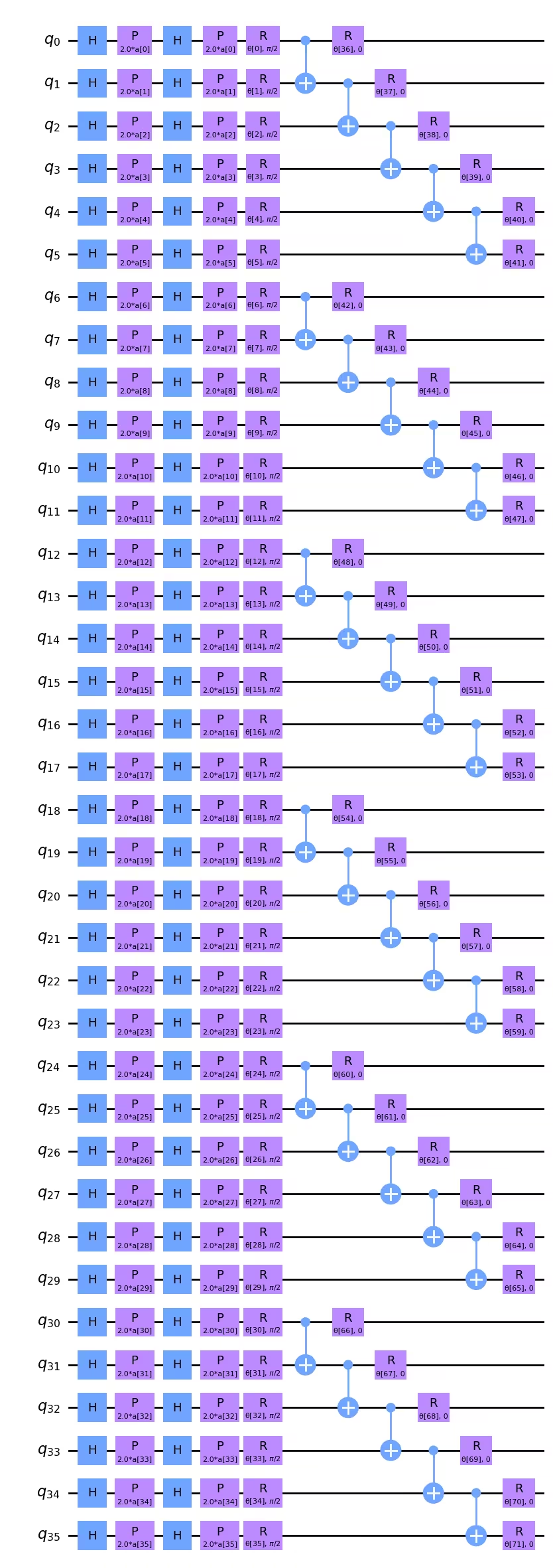
Tu remarqueras peut-être que si minimiser la profondeur de deux qubits était d'une importance capitale, nous pourrions réellement la réduire un peu en changeant l'ordre des portes CNOT. Par exemple, les portes CNOT sur et pourraient être déplacées vers la gauche dans le diagramme du circuit ci-dessus, et pourraient être placées directement en dessous des portes CNOT sur et , par exemple. Pour une profondeur de porte de deux qubits de 5, il n'est pas évident que cela ferait une différence après la transpilation, mais c'est quelque chose à garder à l'esprit. Si l'ordre des portes CNOT est important pour mapper logiquement le problème en question, la profondeur ici est fine. Si l'ordre des portes CNOT n'est pas critique pour modéliser la structure des données de nos images, alors nous pourrions écrire un script pour réorganiser ces portes CNOT et minimiser la profondeur.
Nous devons également redéfinir notre observable avec nos images plus grandes :
from qiskit.quantum_info import SparsePauliOp

observable = SparsePauliOp.from_list([("Z" * (num_qubits), 1)])
Étape 2 des motifs Qiskit : Optimiser le problème pour l'exécution quantique
Nous commençons par sélectionner un backend pour l'exécution. Dans ce cas, nous utiliserons le backend le moins occupé.
from qiskit_ibm_runtime import QiskitRuntimeService

# To run on hardware, select the least busy quantum computer or specify a particular one.
service = QiskitRuntimeService()
backend = service.least_busy(operational=True, simulator=False)
# backend = service.backend("ibm_brisbaneane")

print(backend.name)
ibm_brisbane
Une fois de plus, nous définissons un gestionnaire de passe avec le niveau d'optimisation défini à 3.
from qiskit.circuit.library import XGate
from qiskit.transpiler import PassManager
from qiskit.transpiler.passes import (
    ALAPScheduleAnalysis,
    ConstrainedReschedule,
    PadDynamicalDecoupling,
)
from qiskit.transpiler.preset_passmanagers import generate_preset_pass_manager

target = backend.target

pm = generate_preset_pass_manager(target=target, optimization_level=3)
pm.scheduling = PassManager(
    [
        ALAPScheduleAnalysis(target=target),
        ConstrainedReschedule(
            acquire_alignment=target.acquire_alignment,
            pulse_alignment=target.pulse_alignment,
            target=target,
        ),
        PadDynamicalDecoupling(
            target=target,
            dd_sequence=[XGate(), XGate()],
            pulse_alignment=target.pulse_alignment,
        ),
    ]
)
Maintenant nous appliquons le gestionnaire de passe plusieurs fois. Pour les circuits très larges ou très profonds, il peut y avoir une grande variabilité dans les profondeurs de deux qubits transpilées. Sur de tels circuits, il est important de tester le gestionnaire de passe de nombreuses fois et d'utiliser le meilleur (le plus superficiel) résultat.
# Try pass manager several times, since heuristics can return various transpilations on large
# circuits, and we want the shallowest.

transpiled_qcs = []
transpiled_depths = []
transpiled_2q_depths = []
for i in range(1, 10):
    circuit_ibm = pm.run(full_circuit)
    transpiled_qcs.append(circuit_ibm)
    transpiled_depths.append(circuit_ibm.decompose().depth())
    transpiled_2q_depths.append(
        circuit_ibm.decompose().depth(lambda instr: len(instr.qubits) > 1)
    )
    # print(i)

print(transpiled_depths)
print(transpiled_2q_depths)

# Use the shallowest

minpos = transpiled_2q_depths.index(min(transpiled_2q_depths))
[85, 85, 81, 89, 81, 81, 89, 85, 85]
[10, 10, 10, 10, 10, 10, 10, 10, 10]
Nous voyons que dans ce cas, la profondeur de deux qubits transpilée était toujours 10. Il y avait une variation mineure dans la profondeur d'un seul qubit, et nous utiliserons la plus superficielle. Mais sur ce circuit de 36 qubits, cela n'est pas une amélioration critique. Nous pouvons visualiser ce circuit transpilé, bien qu'à cette échelle, il devient de plus en plus difficile à analyser visuellement.
circuit_ibm = transpiled_qcs[2]
observable_ibm = observable.apply_layout(circuit_ibm.layout)
print(circuit_ibm.decompose().depth())
print(
    f"2+ qubit depth: {circuit_ibm.decompose().depth(lambda instr: len(instr.qubits) > 1)}"
)
81
2+ qubit depth: 10
Étape 3 des motifs Qiskit : Exécuter en utilisant les primitives Qiskit
Pour limiter le temps utilisé sur de vrais ordinateurs quantiques, nous n'effectuerons que quelques étapes d'optimisation ici, et nous le ferons sur un très petit ensemble d'entraînement. Mais la mise à l'échelle de ceci à plus d'étapes d'optimisation et d'ensembles de données de test plus grands devrait être claire à partir des instructions tout au long de la leçon.
# This was run on an Eagle r3 processor on 10-4-24, and took 7 min.

from qiskit_ibm_runtime import EstimatorV2 as Estimator, Session

batch_size = 7
num_epochs = 1
num_samples = len(train_images)

# Globals
circuit = circuit_ibm
observable = observable_ibm
objective_func_vals = []
iter = 0

# Random initial weights for the ansatz
np.random.seed(42)
# weight_params = np.random.rand(len(ansatz.parameters)) * 2 * np.pi
# Or re-load weights from a previous calculation
weight_params = np.array(
    [
        3.35330497,
        5.97351416,
        4.59925358,
        3.76148219,
        0.98029403,
        0.98014248,
        0.3649501,
        6.44234523,
        3.77691701,
        4.44895122,
        0.12933619,
        6.09412333,
        5.23039137,
        1.33416598,
        1.14243996,
        1.15236452,
        1.91161039,
        3.2971419,
        3.71399059,
        1.82984665,
        3.84438512,
        0.87646578,
        1.83559896,
        2.30191935,
        2.86557222,
        4.93340606,
        1.25458737,
        3.23103027,
        3.72225051,
        0.29185655,
        3.81731689,
        1.07143467,
        0.40873121,
        5.96202367,
        6.067245,
        5.07931034,
        1.91394476,
        0.61369199,
        4.2991629,
        2.76555968,
        0.76678884,
        3.11128829,
        0.21606945,
        5.71342859,
        1.62596258,
        4.16275028,
        1.95853845,
        3.26768375,
        3.43508199,
        1.1614748,
        6.09207989,
        4.87030317,
        5.90304595,
        5.62236606,
        3.75671636,
        5.79230665,
        0.55601479,
        1.23139664,
        0.28417144,
        2.04411075,
        2.44213144,
        1.70493625,
        5.20711134,
        2.24154726,
        1.76516358,
        3.40986006,
        0.88545302,
        5.04035228,
        0.46841551,
        6.2007935,
        4.85215699,
        1.24856745,
    ]
)

# Running in a session avoids repeated queuing. This is available to Premium Plan, Flex Plan, and
# On-Prem (IBM Quantum Platform API) Plan users.

with Session(backend=backend) as session:
    estimator = Estimator(mode=session, options={"resilience_level": 1})

    for epoch in range(num_epochs):
        for i in range((num_samples - 1) // batch_size + 1):
            print(f"Epoch: {epoch}, batch: {i}")
            start_i = i * batch_size
            end_i = start_i + batch_size
            train_images_batch = np.array(train_images[start_i:end_i])
            train_labels_batch = np.array(train_labels[start_i:end_i])
            input_params = train_images_batch
            target = train_labels_batch
            iter = 0
            # We can increase maxiter to do a full optimization.
            res = minimize(
                mse_loss_weights,
                weight_params,
                method="COBYLA",
                options={"maxiter": 20},
            )
            weight_params = res["x"]
session.close()

# Open users can carry out the same calculation using a batch, but repeated queuing is possible.
# from qiskit_ibm_runtime import Batch

# with Batch(backend=backend) as batch:
#    estimator = Estimator(
#        mode=batch, options={"resilience_level": 1}
#    )
#
#    for epoch in range(num_epochs):
#        for i in range((num_samples - 1) // batch_size + 1):
#            print(f"Epoch: {epoch}, batch: {i}")
#            start_i = i * batch_size
#            end_i = start_i + batch_size
#            train_images_batch = np.array(train_images[start_i:end_i])
#            train_labels_batch = np.array(train_labels[start_i:end_i])
#            input_params = train_images_batch
#            target = train_labels_batch
#            iter = 0
#            # We can increase maxiter to do a full optimization.
#            res = minimize(
#                mse_loss_weights,
#                weight_params,
#                method="COBYLA",
#                options={"maxiter": 20},
#            )
#            weight_params = res["x"]
# batch.close()
Il est recommandé de sauvegarder les paramètres de poids retournés par ce calcul, au cas où tu déciderais d'itérer davantage.
weight_params
array([3.35330497, 6.97351416, 5.59925358, 3.76148219, 0.98029403,
       0.98014248, 0.3649501 , 6.44234523, 3.77691701, 4.44895122,
       1.12933619, 7.09412333, 5.23039137, 1.33416598, 1.14243996,
       1.15236452, 1.91161039, 3.2971419 , 3.71399059, 1.82984665,
       3.84438512, 0.87646578, 1.83559896, 2.30191935, 2.86557222,
       4.93340606, 1.25458737, 3.23103027, 3.72225051, 0.29185655,
       3.81731689, 1.07143467, 0.40873121, 5.96202367, 6.067245  ,
       5.07931034, 1.91394476, 0.61369199, 4.2991629 , 2.76555968,
       0.76678884, 3.11128829, 0.21606945, 5.71342859, 1.62596258,
       4.16275028, 1.95853845, 3.26768375, 3.43508199, 1.1614748 ,
       6.09207989, 4.87030317, 5.90304595, 5.62236606, 3.75671636,
       5.79230665, 0.55601479, 1.23139664, 0.28417144, 2.04411075,
       2.44213144, 1.70493625, 5.20711134, 2.24154726, 1.76516358,
       3.40986006, 0.88545302, 5.04035228, 0.46841551, 6.2007935 ,
       4.85215699, 1.24856745])
Nous pouvons tracer ces premiers pas d'optimisation, bien que nous ne nous attendions pas à une convergence après aussi peu d'étapes. Ces courbes ont été relativement plates pendant les premiers pas, même en utilisant des simulateurs. Cependant, il convient de noter que l'optimisation actuelle a 72 paramètres libres. Ceci peut être réduit d'au moins un facteur de 2 à 3 sans compromettre les résultats, par exemple, en paramétrisant les qubits avec des données correspondant à un sous-ensemble de lignes et colonnes complètes. En effet, l'espace des paramètres devrait être réduit avant de passer plus de temps de calcul quantique à minimiser la fonction de perte.
obj_func_vals_qc = objective_func_vals
# import matplotlib.pyplot as plt

plt.figure(figsize=(12, 6))
plt.plot(obj_func_vals_qc, label="revised ansatz")
plt.xlabel("iteration")
plt.ylabel("loss")
plt.legend()
plt.show()

Conclusion
En résumé, dans cette leçon, nous avons appris le flux de travail pour la classification binaire d'images en utilisant un réseau de neurones quantiques. Certaines considérations clés dans chaque étape des motifs Qiskit étaient :
Étape 1 : Mapper le problème à un circuit quantique
- Charger les données d'entraînement. Ceci peut être fait « à la main » ou en utilisant une carte de caractéristiques pré-construite comme
z_feature_map. - Construire un ansatz contenant des couches de rotation et d'intrication appropriées à ton problème.
- Monitorer la profondeur du circuit pour assurer des résultats de qualité sur les ordinateurs quantiques.
Étape 2 : Optimiser le problème pour l'exécution quantique
- Sélectionner un backend, généralement le moins occupé.
- Utiliser un gestionnaire de passe pour transpiler à la fois le circuit et les observables à l'architecture du backend choisi.
- Pour les circuits très profonds ou très larges, transpiler plusieurs fois et sélectionner le circuit le plus superficiel.
Étape 3 : Exécuter en utilisant les primitives Qiskit (Runtime)
- Effectuer des essais préliminaires sur simulateurs pour déboguer et optimiser ton ansatz.
- Exécuter sur un ordinateur quantique d'IBM®.
Étape 4 : Post-traiter, retourner le résultat au format classique
- Calculer la précision du modèle sur les données d'entraînement et sur les données de test.
- Monitorer la convergence de l'optimisation classique.