L'algorithme de Deutsch-Jozsa

Pour ce module Qiskit en classe, les étudiants doivent disposer d'un environnement Python fonctionnel avec les packages suivants installés :

• qiskit v2.1.0 ou plus récent
• qiskit-ibm-runtime v0.40.1 ou plus récent
• qiskit-aer v0.17.0 ou plus récent
• qiskit.visualization
• numpy
• pylatexenc

Pour configurer et installer les packages ci-dessus, consulte le guide Installer Qiskit. Pour exécuter des tâches sur de vrais ordinateurs quantiques, les étudiants devront créer un compte IBM Quantum® en suivant les étapes du guide Configurer ton compte IBM Cloud.

Ce module a été testé et a utilisé quatre secondes de temps QPU. Il s'agit d'une estimation uniquement. Ton utilisation réelle peut varier.

# Added by doQumentation — required packages for this notebook
!pip install -q numpy qiskit qiskit-aer qiskit-ibm-runtime

# Uncomment and modify this line as needed to install dependencies
#!pip install 'qiskit>=2.1.0' 'qiskit-ibm-runtime>=0.40.1' 'qiskit-aer>=0.17.0' 'numpy' 'pylatexenc'

Regarde la présentation du module par Dr Katie McCormick ci-dessous, ou clique ici pour la regarder sur YouTube.

---

Introduction

Au début des années 1980, les physiciens quantiques et les informaticiens avaient une vague notion que la mécanique quantique pouvait être exploitée pour effectuer des calculs bien plus puissants que ce que les ordinateurs classiques peuvent faire. Leur raisonnement était le suivant : il est difficile pour un ordinateur classique de simuler des systèmes quantiques, mais un ordinateur quantique devrait pouvoir le faire plus efficacement. Et si un ordinateur quantique pouvait simuler des systèmes quantiques plus efficacement, peut-être y avait-il d'autres tâches qu'il pourrait accomplir plus efficacement qu'un ordinateur classique.

La logique était solide, mais les détails restaient à élaborer. Cela a commencé en 1985, quand David Deutsch a décrit le premier « ordinateur quantique universel ». Dans ce même article, il a fourni le premier exemple de problème pour lequel un ordinateur quantique pouvait résoudre quelque chose plus efficacement qu'un ordinateur classique. Ce premier exemple jouet est désormais connu sous le nom d'« algorithme de Deutsch ». L'amélioration apportée par l'algorithme de Deutsch était modeste, mais Deutsch a travaillé avec Richard Jozsa quelques années plus tard pour élargir davantage l'écart entre les ordinateurs classiques et quantiques.

Ces algorithmes — celui de Deutsch, et l'extension Deutsch-Jozsa — ne sont pas particulièrement utiles, mais ils restent vraiment importants pour plusieurs raisons :

1. Historiquement, ils ont été parmi les premiers algorithmes quantiques dont on a démontré qu'ils surpassaient leurs équivalents classiques. Les comprendre peut nous aider à saisir comment la réflexion de la communauté sur l'informatique quantique a évolué au fil du temps.
2. Ils peuvent nous aider à comprendre certains aspects de la réponse à une question étonnamment subtile : d'où vient la puissance de l'informatique quantique ? Parfois, les ordinateurs quantiques sont comparés à d'énormes processeurs parallèles à échelle exponentielle. Mais ce n'est pas tout à fait exact. Si une partie de la réponse réside dans ce qu'on appelle le « parallélisme quantique », extraire le maximum d'informations en une seule exécution est un art subtil. Les algorithmes de Deutsch et Deutsch-Jozsa montrent comment y parvenir.

Dans ce module, nous allons découvrir l'algorithme de Deutsch, l'algorithme de Deutsch-Jozsa, et ce qu'ils nous enseignent sur la puissance de l'informatique quantique.

Le parallélisme quantique et ses limites

Une partie de la puissance de l'informatique quantique provient du « parallélisme quantique », c'est-à-dire essentiellement la capacité d'effectuer des opérations sur plusieurs entrées en même temps, car les états d'entrée des qubits peuvent être en superposition de plusieurs états classiquement autorisés. CEPENDANT, bien qu'un circuit quantique puisse être capable d'évaluer plusieurs états d'entrée à la fois, il est impossible d'extraire toutes ces informations en une seule opération.

Pour comprendre ce que je veux dire, supposons que nous ayons un bit, $x$, et une fonction appliquée à ce bit, $f(x)$. Il existe quatre fonctions binaires possibles qui prennent un seul bit et retournent un seul bit :

$x$	$f_1(x)$	$f_2(x)$	$f_3(x)$	$f_4(x)$
0	0	0	1	1
1	0	1	0	1

Nous aimerions savoir laquelle de ces fonctions (1 à 4) est notre $f(x)$. Classiquement, nous devrions exécuter la fonction deux fois — une fois pour $x=0$, une fois pour $x=1$. Mais voyons si nous pouvons faire mieux avec un circuit quantique. Nous pouvons en apprendre davantage sur la fonction grâce à la porte suivante :

Ici, la porte $U_f$ calcule $f(x)$, où $x$ est l'état du qubit 0, et l'applique au qubit 1. Ainsi, l'état résultant, $|x\rangle|y\oplus f(x)\rangle$, devient simplement $|x\rangle|f(x)\rangle$ quand $|y\rangle = |0\rangle$. Cela contient toutes les informations dont nous avons besoin pour connaître la fonction $f(x)$ : le qubit 0 nous dit ce qu'est $x$, et le qubit 1 nous dit ce qu'est $f(x)$. Donc, si nous initialisons $|x\rangle = \frac{1}{\sqrt{2}}(|0\rangle+|1\rangle)$, alors l'état final des deux qubits sera : $|y\rangle|x\rangle = \frac{1}{\sqrt{2}}(|f(0)\rangle|0\rangle+|f(1)\rangle|1\rangle)$. Mais comment accéder à ces informations ?

2.1. Essaie avec Qiskit :

Avec Qiskit, nous allons sélectionner aléatoirement l'une des quatre fonctions possibles ci-dessus et exécuter le circuit. Ta tâche est ensuite d'utiliser les mesures du circuit quantique pour découvrir la fonction en un minimum d'exécutions.

Dans cette première expérience et tout au long du module, nous utiliserons un cadre de travail pour l'informatique quantique appelé « Qiskit patterns », qui décompose les flux de travail en les étapes suivantes :

• Étape 1 : Mapper les entrées classiques vers un problème quantique
• Étape 2 : Optimiser le problème pour l'exécution quantique
• Étape 3 : Exécuter en utilisant les Primitives Qiskit Runtime
• Étape 4 : Post-traitement et analyse classique

Commençons par charger quelques packages nécessaires, y compris les primitives Qiskit Runtime. Nous sélectionnerons également l'ordinateur quantique le moins chargé disponible.

Il y a du code ci-dessous pour enregistrer tes identifiants lors de la première utilisation. Assure-toi de supprimer ces informations du notebook après les avoir sauvegardées dans ton environnement, afin que tes identifiants ne soient pas partagés accidentellement quand tu partages le notebook. Consulte Configurer ton compte IBM Cloud et Initialiser le service dans un environnement non fiable pour plus de conseils.

# Load the Qiskit Runtime service
from qiskit_ibm_runtime import QiskitRuntimeService

# Load the Runtime primitive and session
from qiskit_ibm_runtime import SamplerV2 as Sampler

# Syntax for first saving your token.  Delete these lines after saving your credentials.

# QiskitRuntimeService.save_account(channel='ibm_quantum_platform',
# instance = '<YOUR_IBM_INSTANCE_CRN>', token='<YOUR_API_KEY>', overwrite=True, set_as_default=True)
# service = QiskitRuntimeService(channel='ibm_quantum_platform')

# Load saved credentials
service = QiskitRuntimeService()

# Use the least busy backend, or uncomment the loading of a specific backend like "ibm_brisbane".
# backend = service.least_busy(operational=True, simulator=False, min_num_qubits = 127)
backend = service.backend("ibm_brisbane")
print(backend.name)

sampler = Sampler(mode=backend)

ibm_brisbane

La cellule ci-dessous te permettra de basculer entre l'utilisation du simulateur ou du vrai matériel tout au long du notebook. Nous te recommandons de l'exécuter maintenant :

# Load the backend sampler
from qiskit.primitives import BackendSamplerV2

# Load the Aer simulator and generate a noise model based on the currently-selected backend.
from qiskit_aer import AerSimulator
from qiskit_aer.noise import NoiseModel

# Alternatively, load a fake backend with generic properties and define a simulator.

noise_model = NoiseModel.from_backend(backend)

# Define a simulator using Aer, and use it in Sampler.
backend_sim = AerSimulator(noise_model=noise_model)
sampler_sim = BackendSamplerV2(backend=backend_sim)

# You could also define a simulator-based sampler using a generic backend:
# backend_gen = GenericBackendV2(num_qubits=18)
# sampler_gen = BackendSamplerV2(backend=backend_gen)

Maintenant que nous avons chargé les packages nécessaires, nous pouvons procéder au flux de travail Qiskit patterns. Dans l'étape de mapping ci-dessous, nous créons d'abord une fonction qui sélectionne parmi les quatre fonctions possibles prenant un seul bit et retournant un seul bit.

# Step 1: Map

from qiskit import QuantumCircuit

qc = QuantumCircuit(2)

def twobit_function(case: int):
    """
    Generate a valid two-bit function as a `QuantumCircuit`.
    """
    if case not in [1, 2, 3, 4]:
        raise ValueError("`case` must be 1, 2, 3, or 4.")

    f = QuantumCircuit(2)
    if case in [2, 3]:
        f.cx(0, 1)
    if case in [3, 4]:
        f.x(1)
    return f

# first, convert oracle circuit (above) to a single gate for drawing purposes. otherwise, the
# circuit is too large to display

# you may edit the number inside "twobit_function()" to select among the four valid functions:
# blackbox = twobit_function(2).to_gate()

# blackbox.label = "$U_f$"

qc.h(0)
qc.barrier()
qc.compose(twobit_function(2), inplace=True)
qc.measure_all()

qc.draw("mpl")

Dans le circuit ci-dessus, la porte de Hadamard « H » prend le qubit 0, qui est initialement dans l'état $|0\rangle$, et le transforme en l'état de superposition $\frac{1}{\sqrt{2}}(|0\rangle+|1\rangle)$. Ensuite, $U_f$ évalue la fonction $f(x)$ et l'applique au qubit 1.

Nous devons ensuite optimiser et transpiler le circuit pour l'exécuter sur l'ordinateur quantique :

# Step 2: Transpile
from qiskit.transpiler.preset_passmanagers import generate_preset_pass_manager

target = backend.target
pm = generate_preset_pass_manager(target=target, optimization_level=3)

qc_isa = pm.run(qc)

Enfin, nous exécutons notre circuit transpilé sur l'ordinateur quantique et visualisons nos résultats :

# Step 3: Run the job on a real quantum computer

job = sampler.run([qc_isa], shots=1)
# job = sampler_sim.run([qc_isa],shots=1) # uncomment this line to run on simulator instead
res = job.result()
counts = res[0].data.meas.get_counts()

# Step 4: Visualize and analyze results

## Analysis
from qiskit.visualization import plot_histogram

plot_histogram(counts)

Ce qui précède est un histogramme de nos résultats. Selon le nombre de shots que tu as choisi pour exécuter le circuit à l'étape 3 ci-dessus, tu pourrais voir une ou deux barres, représentant les états mesurés des deux qubits dans chaque shot. Comme toujours avec Qiskit et dans ce notebook, nous utilisons la notation « little endian », ce qui signifie que les états des qubits 0 à n sont écrits dans l'ordre croissant de droite à gauche, donc le qubit 0 est toujours le plus à droite.

Ainsi, parce que le qubit 0 était dans un état de superposition, le circuit a évalué la fonction pour les deux $x=0$ et $x=1$ en même temps — quelque chose que les ordinateurs classiques ne peuvent pas faire ! Mais l'inconvénient apparaît quand nous voulons en apprendre davantage sur la fonction $f(x)$ — quand nous mesurons les qubits, nous effondrons leur état. Si tu sélectionnes « shots = 1 » pour n'exécuter le circuit qu'une seule fois, tu ne verras qu'une seule barre dans l'histogramme ci-dessus, et tes informations sur la fonction seront incomplètes.

Vérifie ta compréhension

Lis la ou les question(s) ci-dessous, réfléchis à ta réponse, puis clique sur le triangle pour révéler la solution.

Combien de fois devons-nous exécuter l'algorithme ci-dessus pour apprendre la fonction $f(x)$ ? Est-ce que c'est mieux que le cas classique ? Préfères-tu un ordinateur classique ou quantique pour résoudre ce problème ?

Réponse :

Puisque la mesure va effondrer la superposition et ne retourner qu'une seule valeur, nous devons exécuter le circuit au moins deux fois pour retourner les deux sorties de la fonction $f(0)$ et $f(1)$. Dans le meilleur des cas, cela fonctionne aussi bien que le cas classique, où nous calculons à la fois $f(0)$ et $f(1)$ lors des deux premières requêtes. Mais il y a une chance que nous ayons besoin de l'exécuter plus de deux fois, car la mesure finale est probabiliste et pourrait retourner la même valeur $f(x)$ les deux premières fois. Je préférerais avoir un ordinateur classique dans ce cas.

Ainsi, bien que le parallélisme quantique puisse être puissant lorsqu'il est utilisé de la bonne manière, il est inexact de dire qu'un ordinateur quantique fonctionne comme un énorme processeur parallèle classique. L'acte de mesure effondre les états quantiques, donc nous ne pouvons accéder qu'à une seule sortie du calcul à la fois.

L'algorithme de Deutsch

Bien que le parallélisme quantique seul ne nous donne pas d'avantage sur les ordinateurs classiques, nous pouvons le combiner avec un autre phénomène quantique, l'interférence, pour obtenir une accélération. L'algorithme aujourd'hui connu sous le nom d'« algorithme de Deutsch » est le premier exemple d'un algorithme qui y parvient.

Le problème

Voici le problème :

Étant donné un bit d'entrée, $x = \{0,1\}$, et une fonction d'entrée $f(x) = \{0,1\}$, déterminer si la fonction est équilibrée ou constante. C'est-à-dire que si elle est équilibrée, la sortie de la fonction est 0 la moitié du temps et 1 l'autre moitié. Si elle est constante, la sortie de la fonction est soit toujours 0, soit toujours 1. Rappelle-toi le tableau des quatre fonctions possibles prenant un seul bit et retournant un seul bit :

$x$	$f_1(x)$	$f_2(x)$	$f_3(x)$	$f_4(x)$
0	0	0	1	1
1	0	1	0	1

Les première et dernière fonctions, $f_1(x)$ et $f_4(x)$, sont constantes, tandis que les deux fonctions du milieu, $f_2(x)$ et $f_3(x)$, sont équilibrées.

L'algorithme

La façon dont Deutsch a abordé ce problème s'est faite à travers le « modèle de requête ». Dans le modèle de requête, la fonction d'entrée ($f_i(x)$ ci-dessus) est contenue dans une « boîte noire » — nous n'avons pas accès direct à son contenu, mais nous pouvons interroger la boîte noire et elle nous donnera la sortie de la fonction. On dit parfois qu'un « oracle » fournit cette information. Consulte Leçon 1 : Algorithmes de requête quantique du cours Fondamentaux des algorithmes quantiques pour en savoir plus sur le modèle de requête.

Pour déterminer si un algorithme quantique est plus efficace qu'un algorithme classique dans le modèle de requête, nous pouvons simplement comparer le nombre de requêtes que nous devons effectuer auprès de la boîte noire dans chaque cas. Dans le cas classique, pour savoir si la fonction contenue dans la boîte noire est équilibrée ou constante, nous aurions besoin d'interroger la boîte deux fois pour obtenir à la fois $f(0)$ et $f(1)$.

Dans l'algorithme quantique de Deutsch, cependant, il a trouvé un moyen d'obtenir l'information avec une seule requête ! Il a apporté un ajustement au circuit de « parallélisme quantique » ci-dessus, de sorte qu'il préparait un état de superposition sur les deux qubits, au lieu de seulement sur le qubit 0. Ensuite, les deux sorties de la fonction, $f(0)$ et $f(1)$, ont interféré pour retourner 0 si elles étaient toutes les deux 0 ou toutes les deux 1 (la fonction était constante), et retourner 1 si elles étaient différentes (la fonction était équilibrée). De cette façon, Deutsch pouvait différencier une fonction constante d'une fonction équilibrée avec une seule requête.

Voici un schéma du circuit de l'algorithme de Deutsch :

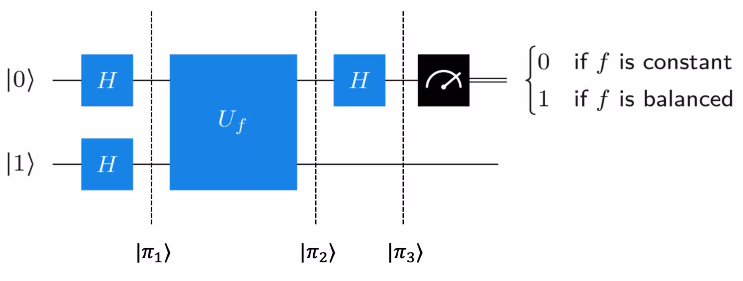
Pour comprendre comment cet algorithme fonctionne, examinons les états quantiques des qubits aux trois points indiqués sur le schéma ci-dessus. Essaie de trouver les états par toi-même avant de cliquer pour voir les réponses :

Vérifie ta compréhension

Lis les questions ci-dessous, réfléchis à tes réponses, puis clique sur les triangles pour révéler les solutions.

Quel est l'état $|\pi_1\rangle$ ?

Réponse :

Appliquer une transformation de Hadamard transforme l'état $|0\rangle$ en $\frac{1}{\sqrt{2}}(|0\rangle+|1\rangle)$ et l'état $|1\rangle$ en $\frac{1}{\sqrt{2}}(|0\rangle-|1\rangle)$. Donc, l'état complet devient : $|\pi_1\rangle = [\frac{|0\rangle-|1\rangle}{\sqrt{2}}][\frac{|0\rangle+|1\rangle}{\sqrt{2}}]$

Quel est l'état $|\pi_2\rangle$ ?

Réponse :

Avant d'appliquer $U_f$, rappelle-toi ce qu'il fait. Il va changer l'état du qubit 1 en fonction de l'état du qubit 0. Il est donc logique de factoriser l'état du qubit 0 : $|\pi_1\rangle = \frac{1}{2} (|0\rangle-|1\rangle)|0\rangle+\frac{1}{2}(|0\rangle-|1\rangle)|1\rangle$. Ensuite, si $f(0)=f(1)$, les deux termes vont se transformer de la même façon et le signe relatif entre les deux termes reste positif, mais si $f(0)\neq f(1)$, alors cela signifie que le deuxième terme va acquérir un signe moins par rapport au premier terme, changeant l'état du qubit 0 de $\frac{1}{\sqrt{2}}(|0\rangle+|1\rangle)$ à $\frac{1}{\sqrt{2}}(|0\rangle-|1\rangle)$. Donc :

$$|\pi_2\rangle = \begin{cases} \pm[\frac{|0\rangle-|1\rangle}{\sqrt{2}}][\frac{|0\rangle+|1\rangle}{\sqrt{2}}] & \text{si} & f(0) = f(1) \\ \pm[\frac{|0\rangle-|1\rangle}{\sqrt{2}}][\frac{|0\rangle-|1\rangle}{\sqrt{2}}] &\text{si} & f(0) \neq f(1) \\ \end{cases}$$

Quel est l'état $|\pi_3\rangle$ ?

Réponse :

Maintenant, l'état du qubit 0 est soit $\frac{1}{\sqrt{2}}(|0\rangle+|1\rangle)$ soit $\frac{1}{\sqrt{2}}(|0\rangle-|1\rangle)$, selon la fonction. Appliquer la transformation de Hadamard donnera soit $|0\rangle$ soit $|1\rangle$, respectivement.

$$|\pi_3\rangle = \begin{cases} \pm[\frac{|0\rangle-|1\rangle}{\sqrt{2}}]|0\rangle & \text{si} & f(0) = f(1) \\ \pm[\frac{|0\rangle-|1\rangle}{\sqrt{2}}]|1\rangle &\text{si} & f(0) \neq f(1) \\ \end{cases}$$

En examinant tes réponses aux questions ci-dessus, note que quelque chose d'un peu surprenant se produit. Bien que $U_f$ ne fasse rien explicitement à l'état du qubit 0, parce qu'il change le qubit 1 en fonction de l'état du qubit 0, il peut arriver que cela provoque un déphasage dans le qubit 0. C'est ce qu'on appelle le phénomène de « phase-kickback », dont il est question plus en détail dans Leçon 1 : Algorithmes de requête quantique du cours Fondamentaux des algorithmes quantiques.

Maintenant que nous comprenons comment cet algorithme fonctionne, implémentons-le avec Qiskit.

## Deutsch's algorithm:

## Step 1: Map the problem

# first, convert oracle circuit (above) to a single gate for drawing purposes.
# otherwise, the circuit is too large to display
blackbox = twobit_function(
    3
    # you may edit the number (1-4) inside "twobit_function()" to select among the four valid functions
).to_gate()
blackbox.label = "$U_f$"

qc_deutsch = QuantumCircuit(2, 1)

qc_deutsch.x(1)
qc_deutsch.h(range(2))

qc_deutsch.barrier()
qc_deutsch.compose(twobit_function(2), inplace=True)
qc_deutsch.barrier()

qc_deutsch.h(0)
qc_deutsch.measure(0, 0)

qc_deutsch.draw("mpl")

# Step 2: Transpile
from qiskit.transpiler.preset_passmanagers import generate_preset_pass_manager

target = backend.target
pm = generate_preset_pass_manager(target=target, optimization_level=3)

qc_isa = pm.run(qc_deutsch)

# Step 3: Run the job on a real quantum computer

job = sampler.run([qc_isa], shots=1)
# job = sampler_sim.run([qc_isa],shots=1) # uncomment this line to run on simulator instead
res = job.result()
counts = res[0].data.c.get_counts()

# Step 4: Visualize and analyze results

## Analysis
print(counts)
if "1" in counts:
    print("balanced")
else:
    print("constant")

{'1': 1}
balanced

L'algorithme de Deutsch-Jozsa

L'algorithme de Deutsch a été une première étape importante dans la démonstration de la façon dont un ordinateur quantique pourrait être plus efficace qu'un ordinateur classique, mais ce n'était qu'une amélioration modeste : il ne nécessitait qu'une seule requête, contre deux dans le cas classique. En 1992, Deutsch et son collègue Richard Jozsa ont étendu l'algorithme original à deux qubits à un plus grand nombre de qubits. Le problème restait le même : déterminer si une fonction est équilibrée ou constante. Mais cette fois, la fonction passe de $n$ bits à un seul bit. Soit la fonction retourne 0 et 1 un nombre égal de fois (elle est équilibrée), soit la fonction retourne toujours 1 ou toujours 0 (elle est constante).

Voici un schéma du circuit de l'algorithme :

Cet algorithme fonctionne de la même façon que l'algorithme de Deutsch : le phase-kickback permet de lire l'état du qubit 0 pour déterminer si la fonction est constante ou équilibrée. C'est un peu plus difficile à voir que dans le cas de l'algorithme de Deutsch à deux qubits, car les états incluront des sommes sur les $n$ qubits, et donc le calcul de ces états sera laissé comme exercice optionnel pour toi à la fin du module. L'algorithme retournera une chaîne de bits de tous les 0 si la fonction est constante, et une chaîne de bits contenant au moins un 1 si la fonction est équilibrée.

Pour voir comment l'algorithme fonctionne dans Qiskit, nous devons d'abord générer notre oracle : la fonction aléatoire garantie d'être soit constante soit équilibrée. Le code ci-dessous générera une fonction équilibrée 50% du temps, et une fonction constante 50% du temps. Ne t'inquiète pas si tu ne suis pas entièrement le code — il est complexe et n'est pas nécessaire à notre compréhension de l'algorithme quantique.

from qiskit import QuantumCircuit
import numpy as np

def dj_function(num_qubits):
    """
    Create a random Deutsch-Jozsa function.
    """

    qc_dj = QuantumCircuit(num_qubits + 1)
    if np.random.randint(0, 2):
        # Flip output qubits with 50% chance
        qc_dj.x(num_qubits)
    if np.random.randint(0, 2):
        # return constant circuit with 50% chance.
        return qc_dj

    # If the "if" statement above was "TRUE" then we've returned the constant
    # function and the function is complete. If not, we proceed in creating our
    # balanced function. Everything below is to produce the balanced function:

    # select half of all possible states at random:
    on_states = np.random.choice(
        range(2**num_qubits),  # numbers to sample from
        2**num_qubits // 2,  # number of samples
        replace=False,  # makes sure states are only sampled once
    )

    def add_cx(qc_dj, bit_string):
        for qubit, bit in enumerate(reversed(bit_string)):
            if bit == "1":
                qc_dj.x(qubit)
        return qc_dj

    for state in on_states:
        # qc_dj.barrier()  # Barriers are added to help visualize how the functions are created.
        # They can safely be removed.
        qc_dj = add_cx(qc_dj, f"{state:0b}")
        qc_dj.mcx(list(range(num_qubits)), num_qubits)
        qc_dj = add_cx(qc_dj, f"{state:0b}")

    # qc_dj.barrier()

    return qc_dj

n = 3  # number of input qubits

oracle = dj_function(n)

display(oracle.draw("mpl"))

Voici la fonction oracle, qui est soit équilibrée soit constante. En la regardant, peux-tu voir si la sortie du dernier qubit dépend des valeurs entrées pour les $n$ premiers qubits ? Si la sortie du dernier qubit dépend des $n$ premiers qubits, peux-tu dire si cette sortie dépendante est équilibrée ou non ?

Nous pouvons déterminer si la fonction est équilibrée ou constante en regardant le circuit ci-dessus, mais rappelle-toi que, pour les besoins de ce problème, nous considérons cette fonction comme une « boîte noire ». Nous ne pouvons pas regarder à l'intérieur de la boîte pour voir le schéma du circuit. Au lieu de cela, nous devons interroger la boîte.

Pour interroger la boîte, nous utilisons l'algorithme de Deutsch-Jozsa et déterminons si la fonction est constante ou équilibrée :

blackbox = oracle.to_gate()
blackbox.label = "$U_f$"

qc_dj = QuantumCircuit(n + 1, n)
qc_dj.x(n)
qc_dj.h(range(n + 1))
qc_dj.barrier()
qc_dj.compose(blackbox, inplace=True)
qc_dj.barrier()
qc_dj.h(range(n))
qc_dj.measure(range(n), range(n))

qc_dj.decompose().decompose()

qc_dj.draw("mpl")

# Step 1: Map the problem

qc_dj = QuantumCircuit(n + 1, n)
qc_dj.x(n)
qc_dj.h(range(n + 1))
qc_dj.barrier()
qc_dj.compose(oracle, inplace=True)
qc_dj.barrier()
qc_dj.h(range(n))
qc_dj.measure(range(n), range(n))

qc_dj.decompose().decompose()

qc_dj.draw("mpl")

# Step 2: Transpile
from qiskit.transpiler.preset_passmanagers import generate_preset_pass_manager

target = backend.target
pm = generate_preset_pass_manager(target=target, optimization_level=3)

qc_isa = pm.run(qc_dj)

# Step 3: Run the job on a real quantum computer

job = sampler.run([qc_isa], shots=1)
# job = sampler_sim.run([qc_isa],shots=1) # uncomment this line to run on simulator instead
res = job.result()
counts = res[0].data.c.get_counts()

# Step 4: Visualize and analyze results

## Analysis
print(counts)

if (
    "0" * n in counts
):  # The D-J algorithm returns all zeroes if the function was constant
    print("constant")
else:
    print("balanced")  # anything other than all zeroes means the function is balanced.

{'110': 1}
balanced

Ci-dessus, la première ligne de la sortie est la chaîne de bits des résultats de mesure. La deuxième ligne indique si la chaîne de bits implique que la fonction était équilibrée ou constante. Si la chaîne de bits contenait tous des zéros, alors elle était constante ; sinon, elle était équilibrée. Donc, avec une seule exécution du circuit quantique ci-dessus, nous pouvons déterminer si la fonction est constante ou équilibrée !

Vérifie ta compréhension

Lis les questions ci-dessous, réfléchis à tes réponses, puis clique sur les triangles pour révéler les solutions.

Combien de requêtes faudrait-il à un ordinateur classique pour déterminer avec une certitude à 100% si une fonction est constante ou équilibrée ? Rappelle-toi que classiquement, une seule requête te permet uniquement d'appliquer la fonction à une seule chaîne de bits.

Réponse :

Il y a $2^n$ chaînes de bits possibles à vérifier, et dans le pire des cas, tu devrais en tester $2^n/2+1$. Par exemple, si la fonction était constante, et que tu continuais à mesurer « 1 » comme sortie de la fonction, alors tu ne pourrais pas être certain qu'elle était vraiment constante avant d'avoir vérifié plus de la moitié des résultats. Avant cela, tu pourrais avoir simplement été très malchanceux en continuant à mesurer « 1 » sur une fonction équilibrée. C'est comme lancer une pièce encore et encore et qu'elle tombe sur pile à chaque fois. C'est peu probable, mais pas impossible.

Comment ta réponse ci-dessus changerait-elle si tu devais simplement mesurer jusqu'à ce qu'un résultat (équilibré ou constant) soit plus probable que l'autre ? Combien de requêtes cela prendrait-il dans ce cas ?

Réponse :

Dans ce cas, tu pourrais simplement mesurer deux fois. Si les deux mesures sont différentes, tu sais que la fonction est équilibrée. Si les deux mesures sont identiques, elle pourrait être équilibrée ou constante. La probabilité qu'elle soit équilibrée avec cet ensemble de mesures est : $\frac{1}{2}\frac{2^n /2 - 1}{2^n-1}$. C'est inférieur à 1/2, donc il est plus probable que la fonction soit constante dans ce cas.

Ainsi, l'algorithme de Deutsch-Jozsa a démontré une accélération exponentielle par rapport à un algorithme classique déterministe (qui retourne la réponse avec une certitude à 100%), mais aucune accélération significative par rapport à un algorithme probabiliste (qui retourne un résultat susceptible d'être la bonne réponse).

Le problème de Bernstein-Vazirani

En 1997, Ethan Bernstein et Umesh Vazirani ont utilisé l'algorithme de Deutsch-Jozsa pour résoudre un problème plus spécifique et restreint par rapport au problème Deutsch-Jozsa. Plutôt que de simplement essayer de distinguer entre deux classes de fonctions différentes, comme dans le cas D-J, Bernstein et Vazirani ont utilisé l'algorithme de Deutsch-Jozsa pour apprendre réellement une chaîne encodée dans une fonction. Voici le problème :

La fonction $f:\{0,1\}^n \rightarrow \{0,1\}$ prend toujours une chaîne de $n$ bits et retourne un seul bit. Mais maintenant, au lieu de promettre que la fonction est équilibrée ou constante, on nous promet que la fonction est le produit scalaire entre la chaîne d'entrée $x$ et une chaîne secrète de $n$ bits $s$, modulo 2. (Ce produit scalaire modulo 2 est appelé le « produit scalaire binaire ».) Le problème consiste à trouver quelle est la chaîne secrète de $n$ bits.

Écrit autrement, on nous donne une fonction boîte noire $f: {0,1}^n \rightarrow {0,1}$ qui satisfait $f(x) = s \cdot x$ pour une certaine chaîne $s$, et nous voulons apprendre la chaîne $s$.

Regardons comment l'algorithme D-J résout ce problème :

1. D'abord, une porte de Hadamard est appliquée aux $n$ qubits d'entrée, et une porte NOT plus un Hadamard est appliquée au qubit de sortie, donnant l'état :

$$|\Psi\rangle = |-\rangle_{n} \otimes |+\rangle_{n-1} \otimes |+\rangle_{n-2} \otimes ... \otimes |+\rangle_0$$

L'état des qubits 1 à $n$ peut s'écrire plus simplement comme une somme sur tous les $2^n$ états de base à $n$ qubits $|00...00\rangle, |00...01\rangle, |000...11\rangle, ..., |111...11\rangle$. Nous appelons l'ensemble de ces états de base $\Sigma^n$. (Voir Fondamentaux des algorithmes quantiques pour plus de détails.)

$$|\Psi\rangle = |-\rangle \otimes \frac{1}{\sqrt{2^n}}\sum\limits_{x \in \Sigma^n}{|x\rangle}$$

2. Ensuite, la porte $U_f$ est appliquée aux qubits. Cette porte prend les n premiers qubits en entrée (qui sont maintenant en superposition égale de toutes les chaînes de n bits possibles) et applique la fonction $f(x)=s \cdot x$ au qubit de sortie, de sorte que ce qubit est maintenant dans l'état : $|- \oplus f(x)\rangle$. Grâce au mécanisme de phase kickback, l'état de ce qubit reste inchangé, mais certains des termes dans l'état des qubits d'entrée acquièrent un signe moins :

$$|\Psi\rangle = |-\rangle \otimes \frac{1}{\sqrt{2^n}}\sum\limits_{x \in \Sigma^n}{(-1)^{f(x)}|x\rangle}$$

3. Maintenant, la couche suivante de Hadamards est appliquée aux qubits 0 à $n-1$. Suivre les signes moins dans ce cas peut être délicat. Il est utile de savoir qu'appliquer une couche de Hadamards à $n$ qubits dans un état de base standard $|x\rangle$ peut s'écrire comme :

$$H^{\otimes n} |x\rangle = \frac{1}{\sqrt{2^n}}\sum\limits_{y \in \Sigma^n}{(-1)^{x \cdot y}|y\rangle}$$

Donc l'état devient :

$$|\Psi\rangle = |-\rangle \otimes \frac{1}{2^n}\sum\limits_{x \in \Sigma^n}\sum\limits_{y \in \Sigma^n}{(-1)^{(s \cdot x) + (x \cdot y)}|y\rangle}$$

4. L'étape suivante est de mesurer les $n$ premiers bits. Mais que va-t-on mesurer ? Il s'avère que l'état ci-dessus se simplifie en : $|\Psi\rangle = |-\rangle \otimes |s\rangle$, mais ce n'est pas du tout évident. Si tu veux suivre les calculs, consulte le cours Fondamentaux des algorithmes quantiques de John Watrous. L'essentiel est que le mécanisme de phase kickback conduit les qubits d'entrée à être dans l'état $|s\rangle$. Donc, pour découvrir quelle était la chaîne secrète $s$, il suffit de mesurer les qubits !

Vérifie ta compréhension

Lis les questions ci-dessous, réfléchis à tes réponses, puis clique sur les triangles pour révéler les solutions.

Vérifie que l'état de l'étape 3 ci-dessus est bien l'état $|s\rangle$ pour le cas particulier de $n=1$.

Réponse :

Quand tu écris explicitement les deux sommations, tu devrais obtenir un état avec quatre termes (omettons l'état de sortie $|-\rangle$ pour cela) :

$$|\Psi\rangle = \frac{1}{2}[|0\rangle + (-1)^s |0\rangle + |1\rangle + (-1)^{(s+1)} |1\rangle]$$

Si $s=0$, alors les deux premiers termes s'additionnent de façon constructive et les deux derniers termes s'annulent, nous laissant avec $|\Psi\rangle = |0\rangle$. Si $s=1$, alors les deux derniers termes s'additionnent de façon constructive et les deux premiers termes s'annulent, nous laissant avec $|\Psi\rangle = |1\rangle$. Donc, dans les deux cas, $|\Psi\rangle = |s\rangle$. Espérons que ce cas le plus simple te donne une idée de comment fonctionne le cas général avec $n$ qubits : tous les termes qui ne sont pas $|s\rangle$ interfèrent et s'annulent, ne laissant que l'état $|s\rangle$.

Comment le même algorithme peut-il résoudre à la fois les problèmes de Bernstein-Vazirani et Deutsch-Jozsa ? Pour comprendre cela, réfléchis aux fonctions de Bernstein-Vazirani, qui sont de la forme $f(x) = s \cdot x$. Ces fonctions sont-elles aussi des fonctions de Deutsch-Jozsa ? C'est-à-dire, détermine si les fonctions de cette forme satisfont la promesse du problème Deutsch-Jozsa : qu'elles sont soit constantes soit équilibrées. Comment cela nous aide-t-il à comprendre comment le même algorithme résout deux problèmes différents ?

Réponse :

Chaque fonction de Bernstein-Vazirani de la forme $f(x) = s \cdot x$ satisfait également la promesse du problème Deutsch-Jozsa : si s=00...00, alors la fonction est constante (retourne toujours 0 pour toute chaîne x). Si s est une autre chaîne quelconque, alors la fonction est équilibrée. Donc, appliquer l'algorithme de Deutsch-Jozsa à l'une de ces fonctions résout simultanément les deux problèmes ! Il retourne la chaîne, et si cette chaîne est 00...00 alors on sait qu'elle est constante ; s'il y a au moins un « 1 » dans la chaîne, on sait qu'elle est équilibrée.

Nous pouvons également vérifier que cet algorithme résout bien le problème de Bernstein-Vazirani en le testant expérimentalement. D'abord, nous créons la fonction B-V qui se trouve à l'intérieur de la boîte noire :

# Step 1: Map the problem

def bv_function(s):
    """
    Create a Bernstein-Vazirani function from a string of 1s and 0s.
    """
    qc = QuantumCircuit(len(s) + 1)
    for index, bit in enumerate(reversed(s)):
        if bit == "1":
            qc.cx(index, len(s))
    return qc

display(bv_function("1000").draw("mpl"))

string = "1000"  # secret string that we'll pretend we don't know or have access to
n = len(string)

qc = QuantumCircuit(n + 1, n)
qc.x(n)
qc.h(range(n + 1))
qc.barrier()
# qc.compose(oracle, inplace = True)
qc.compose(bv_function(string), inplace=True)
qc.barrier()
qc.h(range(n))
qc.measure(range(n), range(n))

qc.draw("mpl")

# Step 2: Transpile
from qiskit.transpiler.preset_passmanagers import generate_preset_pass_manager

target = backend.target
pm = generate_preset_pass_manager(target=target, optimization_level=3)

qc_isa = pm.run(qc)

# Step 3: Run the job on a real quantum computer

job = sampler.run([qc_isa], shots=1)
# job = sampler_sim.run([qc_isa],shots=1) # uncomment this line to run on simulator instead
res = job.result()
counts = res[0].data.c.get_counts()

# Step 4: Visualize and analyze results

## Analysis
print(counts)

{'0000': 1}

Ainsi, avec une seule requête, l'algorithme de Deutsch-Jozsa retournera la chaîne $s$ utilisée dans la fonction : $f(x)=x \cdot s$ quand nous l'appliquons au problème de Bernstein-Vazirani. Avec un algorithme classique, il faudrait $n$ requêtes pour résoudre le même problème.

Conclusion

Nous espérons qu'en examinant ces exemples simples, nous t'avons donné une meilleure intuition sur la façon dont les ordinateurs quantiques sont capables d'exploiter la superposition, l'intrication et l'interférence pour atteindre leur puissance par rapport aux ordinateurs classiques.

L'algorithme de Deutsch-Jozsa revêt une grande importance historique car il a été le premier à démontrer une quelconque accélération par rapport à un algorithme classique, mais ce n'était qu'une accélération polynomiale. L'algorithme de Deutsch-Jozsa n'est que le début de l'histoire.

Après avoir utilisé l'algorithme pour résoudre leur problème, Bernstein et Vazirani s'en sont servis comme base pour un problème récursif plus complexe appelé le problème d'échantillonnage de Fourier récursif. Leur solution offrait une accélération super-polynomiale par rapport aux algorithmes classiques. Et même avant Bernstein et Vazirani, Peter Shor avait déjà trouvé son fameux algorithme qui permettait aux ordinateurs quantiques de factoriser de grands nombres exponentiellement plus rapidement que n'importe quel algorithme classique. Ces résultats ont collectivement montré la promesse passionnante des futurs ordinateurs quantiques, et ont poussé physiciens et ingénieurs à faire de cet avenir une réalité.

Questions

Les enseignants peuvent demander des versions de ces notebooks avec les corrigés et des conseils sur leur placement dans les programmes courants en remplissant ce court sondage sur la façon dont les notebooks sont utilisés.

Concepts clés

• les algorithmes de Deutsch et Deutsch-Jozsa utilisent le parallélisme quantique combiné à l'interférence pour trouver une réponse à un problème plus rapidement qu'un ordinateur classique.
• le mécanisme de phase kickback est un phénomène quantique contre-intuitif qui transfère des opérations sur un qubit vers la phase d'un autre qubit. Les algorithmes de Deutsch et Deutsch-Jozsa utilisent ce mécanisme.
• L'algorithme de Deutsch-Jozsa offre une accélération polynomiale par rapport à tout algorithme classique déterministe.
• L'algorithme de Deutsch-Jozsa peut être appliqué à un problème différent, appelé le problème de Bernstein-Vazirani, pour trouver une chaîne cachée encodée dans une fonction.

Vrai/faux

1. V/F L'algorithme de Deutsch est un cas particulier de l'algorithme de Deutsch-Jozsa où l'entrée est un seul qubit.
2. V/F Les algorithmes de Deutsch et Deutsch-Jozsa utilisent la superposition quantique et l'interférence pour atteindre leur efficacité.
3. V/F L'algorithme de Deutsch-Jozsa nécessite plusieurs évaluations de la fonction pour déterminer si une fonction est constante ou équilibrée.
4. V/F L'« algorithme de Bernstein-Vazirani » est en réalité le même que l'algorithme de Deutsch-Jozsa, appliqué à un problème différent.
5. V/F L'algorithme de Bernstein-Vazirani peut trouver plusieurs chaînes secrètes simultanément.

Réponses courtes

1. Combien de temps prendrait un algorithme classique pour résoudre le problème Deutsch-Jozsa dans le pire des cas ?

2. Combien de temps prendrait un algorithme classique pour résoudre le problème Bernstein-Vazirani ? Quelle accélération l'algorithme DJ offre-t-il dans ce cas ?

3. Décris le mécanisme de phase kickback et comment il fonctionne pour résoudre les problèmes Deutsch-Jozsa et Bernstein-Vazirani.

Problème défi

1. L'algorithme de Deutsch-Jozsa : Rappelle-toi que tu avais une question ci-dessus te demandant de calculer les états intermédiaires des qubits $\pi_1$ et $\pi_2$ de l'algorithme de Deutsch. Fais de même pour les états intermédiaires à $n+1$ qubits $\pi_1$ et $\pi_2$ de l'algorithme de Deutsch-Jozsa, pour le cas particulier de $n=2$. Ensuite, vérifie que $\pi_3 = |-\rangle \otimes \sum\limits_{x_0...x_n}(-1)^{f(x_0...x_n)}|x_0 ... x_n\rangle$, à nouveau, pour le cas particulier de $n=2$.