Transformée de Fourier quantique

Pour ce module Qiskit en classe, les étudiants doivent disposer d'un environnement Python fonctionnel avec les packages suivants installés :

• qiskit v2.1.0 ou plus récent
• qiskit-ibm-runtime v0.40.1 ou plus récent
• qiskit-aer v0.17.0 ou plus récent
• qiskit.visualization
• numpy
• pylatexenc

Pour configurer et installer les packages ci-dessus, consulte le guide Installer Qiskit. Pour exécuter des jobs sur de vrais ordinateurs quantiques, les étudiants devront créer un compte IBM Quantum® en suivant les étapes du guide Configurer ton compte IBM Cloud.

Ce module a été testé et a utilisé 13 secondes de temps QPU. Il s'agit d'une estimation de bonne foi ; ton utilisation réelle peut varier.

# Added by doQumentation — required packages for this notebook
!pip install -q numpy qiskit qiskit-aer qiskit-ibm-runtime

# Uncomment and modify this line as needed to install dependencies
#!pip install 'qiskit>=2.1.0' 'qiskit-ibm-runtime>=0.40.1' 'qiskit-aer>=0.17.0' 'numpy' 'pylatexenc'

Introduction

Une transformée de Fourier est un outil omniprésent avec des applications en mathématiques, physique, traitement du signal, compression de données et d'innombrables autres domaines. Une version quantique de la transformée de Fourier, appelée à juste titre la transformée de Fourier quantique, constitue la base de certains des algorithmes quantiques les plus importants.

Aujourd'hui, après un rappel de la transformée de Fourier classique, on va parler de la façon dont on implémente la transformée de Fourier quantique sur un ordinateur quantique. Ensuite, on va aborder l'une des applications de la transformée de Fourier quantique à un algorithme appelé l'algorithme d'estimation de phase. L'estimation de phase quantique est une sous-routine dans le célèbre algorithme de factorisation de Shor, parfois désigné comme le « joyau de la couronne » de l'informatique quantique. Ce module prépare le terrain pour un autre module entièrement consacré à l'algorithme de Shor, mais il est aussi conçu pour être autonome. La transformée de Fourier quantique est un algorithme fascinant et utile en soi !

La transformée de Fourier classique

Avant de plonger dans la transformée de Fourier quantique, rappelons-nous d'abord la version classique. La transformée de Fourier est une méthode de passage d'une « base » à une autre. On peut penser à deux bases comme deux perspectives différentes sur un même problème — toutes deux sont des façons valides d'exprimer une fonction, mais l'une ou l'autre peut être plus éclairante selon le problème à résoudre. Quelques exemples de paires de bases reliées par la transformée de Fourier : position et quantité de mouvement, temps et fréquence.

Voyons un exemple de la façon dont la transformée de Fourier peut nous aider à déterminer quelle note joue un instrument à partir de sa forme d'onde audio. Généralement, on voit les formes d'onde représentées dans la base temporelle — c'est-à-dire que l'amplitude de l'onde est exprimée en fonction du temps.

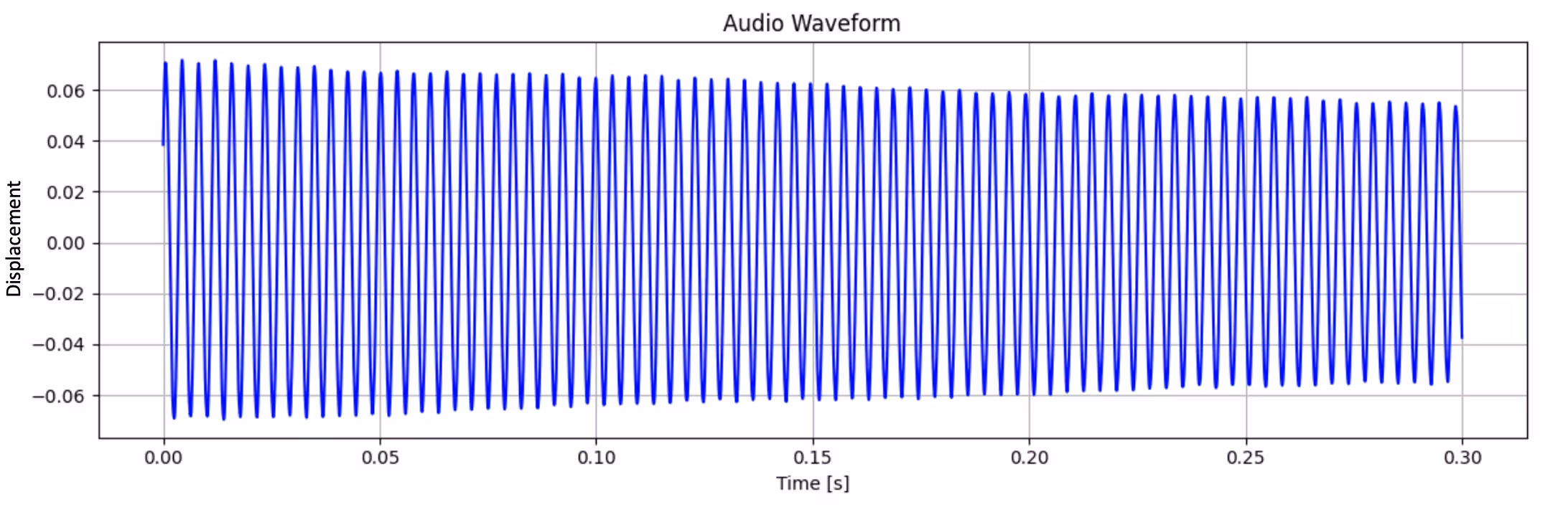
On peut appliquer la transformée de Fourier à cette forme d'onde pour passer de la base temporelle à la base fréquentielle :

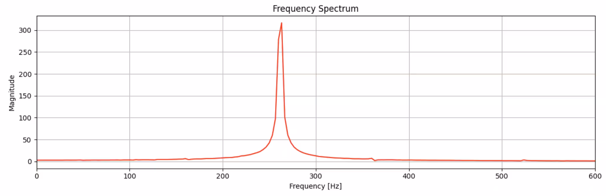
Dans la base fréquentielle, on voit clairement un pic à environ 260 Hz. C'est un do central !

Tu aurais peut-être pu déterminer qu'un do central était joué sans utiliser de transformée de Fourier, mais que se passe-t-il si plusieurs notes sont jouées en même temps ? La forme d'onde devient alors plus complexe lorsqu'on la trace dans la base temporelle :

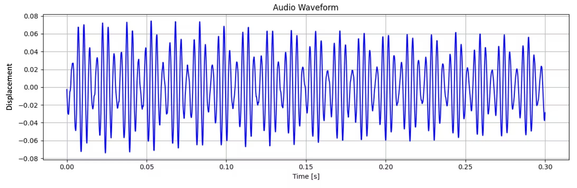
Mais le spectre fréquentiel identifie clairement trois pics :

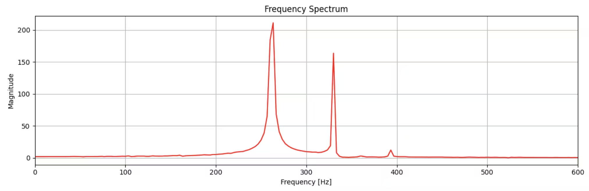
C'était un accord de do majeur, jouant les notes do, mi et sol.

Ce type d'analyse de Fourier peut nous aider à extraire les composantes fréquentielles de tout signal complexe.

Transformée de Fourier discrète

La transformée de Fourier est utile pour de nombreuses applications de traitement du signal. Mais dans la plupart de ces applications réelles (y compris l'exemple musical que l'on vient d'utiliser), on veut transformer un ensemble discret de $N$ points de données — pas une fonction continue. Dans ce cas, on utilise la transformée de Fourier discrète. La transformée de Fourier discrète (DFT) agit sur un vecteur $(x_0, ..., x_{N-1})$ et le fait correspondre au vecteur $(y_0, ..., y_{N-1})$ selon la formule :

$y_k = \frac{1}{\sqrt{N}}\sum_{j=0}^{N-1}x_j\omega_N^{jk}$

où l'on prend $\omega_N^{jk} = e^{2\pi i \frac{jk}{N}}$. (Note qu'il existe d'autres conventions avec un signe moins dans l'exponentielle, fais attention quand tu rencontres la DFT.) Rappelle-toi que $e^{2\pi i \frac{jk}{N}}$ est une fonction périodique, de période $\frac{N}{k}$. Ainsi, en multipliant par cette fonction, la transformée de Fourier est essentiellement une façon de décomposer la fonction (discrète) $\{x_{j}\}$ en une combinaison linéaire de ses fonctions périodiques constitutives, chacune de période $\frac{N}{k}$.

La transformée de Fourier quantique

Maintenant qu'on a vu comment la transformée de Fourier permet de représenter une fonction comme une combinaison linéaire d'un nouvel ensemble de « fonctions de base », on peut aborder les transformations de base sur les états de qubits. Par exemple, l'état d'un seul qubit $|\psi\rangle$ peut être exprimé dans la base computationnelle $|\psi\rangle = c_0 |0\rangle + c_1 |1\rangle$, avec les états de base $|0\rangle$ et $|1\rangle$, ou dans la base $X$ : $|\psi\rangle = c_+ |+\rangle + c_- |-\rangle$ avec les états de base $|+\rangle = \frac{1}{\sqrt{2}} (|0\rangle + |1\rangle)$ et $|-\rangle = \frac{1}{\sqrt{2}} (|0\rangle - |1\rangle)$. Les deux sont également valides, mais l'une peut être plus naturelle que l'autre selon le type de problème à résoudre.

Les états de qubits peuvent aussi être exprimés dans la base de Fourier, où un état est exprimé en termes de combinaison linéaire des états de base de Fourier $|\phi_y\rangle$, plutôt que des états de base computationnels habituels $|x\rangle$. Pour ce faire, il faut appliquer une transformée de Fourier quantique (QFT) :

$| \phi_y \rangle = \frac{1}{\sqrt{N}}\sum_{x=0}^{N-1}\omega_N^{y x} \vert x \rangle$

avec $\omega_N^{yx} = e^{\frac{2\pi i y x}{N}}$ comme précédemment, et $N$ est le nombre d'états de base dans ton système quantique. Comme on travaille maintenant avec des qubits, $m$ qubits donnent $2^m$ états de base, donc $N=2^m$. Ici, les états de base sont écrits comme un seul nombre $|x\rangle$ où $x$ va de $0$ à $N-1$, mais tu verras plus souvent les états de base exprimés comme $|00...00\rangle$, $|00...01\rangle$, $|00...11\rangle$, ..., $|11...11\rangle$, où chaque chiffre binaire représente l'état du qubit 0 au qubit $m-1$, de droite à gauche. Il y a une façon simple de convertir ces états binaires en un seul nombre : traite-les simplement comme des nombres binaires ! Ainsi, $|00...00\rangle = |0\rangle$, $|00...01\rangle = |1\rangle$, $|00...10\rangle = |2\rangle$, $|00...11\rangle = |3\rangle$, et ainsi de suite, jusqu'à $|11...11\rangle = |2^m -1\rangle = |N-1\rangle$.

Développe ton intuition pour les états de base de Fourier

On vient de passer en revue ce que sont les états de base computationnels et comment ils sont ordonnés : ce sont les états où chaque qubit est soit en $0$ soit en $1$, ordonnés de l'état où tous les qubits sont à $0$, $|00...00\rangle$, à l'état où ils sont tous à $1$, $|11...11\rangle$.

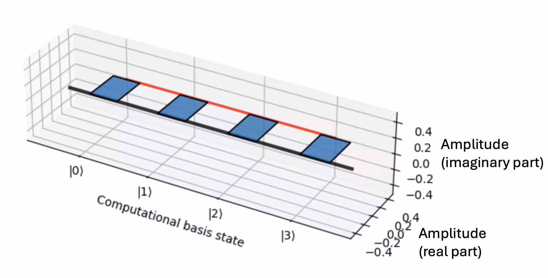
Mais comment comprendre les états de base de Fourier ? Tous les états de base de Fourier sont des superpositions égales de tous les états de base computationnels, mais chaque état diffère des autres par la périodicité de la phase de ses composantes. Pour comprendre cela de manière concrète, examinons les quatre états de base de Fourier d'un système à deux qubits. L'état de Fourier le plus bas est celui dont la phase ne varie pas du tout :

$|\phi_0\rangle = \frac{1}{2} (|00\rangle + |01\rangle + |10\rangle + |11\rangle)$

On peut visualiser cet état en traçant l'amplitude complexe de chacun des termes. La ligne rouge guide l'œil pour montrer comment la phase de cette amplitude s'enroule dans le plan complexe en fonction de l'état de base computationnel. Pour $|\phi_0\rangle$, la phase reste constante :

L'état de base de Fourier suivant est celui dont les phases des composantes s'enroulent de $0$ à $2\pi$ exactement une fois :

$|\phi_1\rangle = \frac{1}{2} (|00\rangle + e^{i\pi/2}|01\rangle + e^{i\pi}|10\rangle + e^{3i\pi/2}|11\rangle) = \frac{1}{2}(|00\rangle + i|01\rangle - |10\rangle - i|11\rangle)$

Et on peut voir cet enroulement dans le graphique de l'amplitude complexe en fonction de l'état de base computationnel :

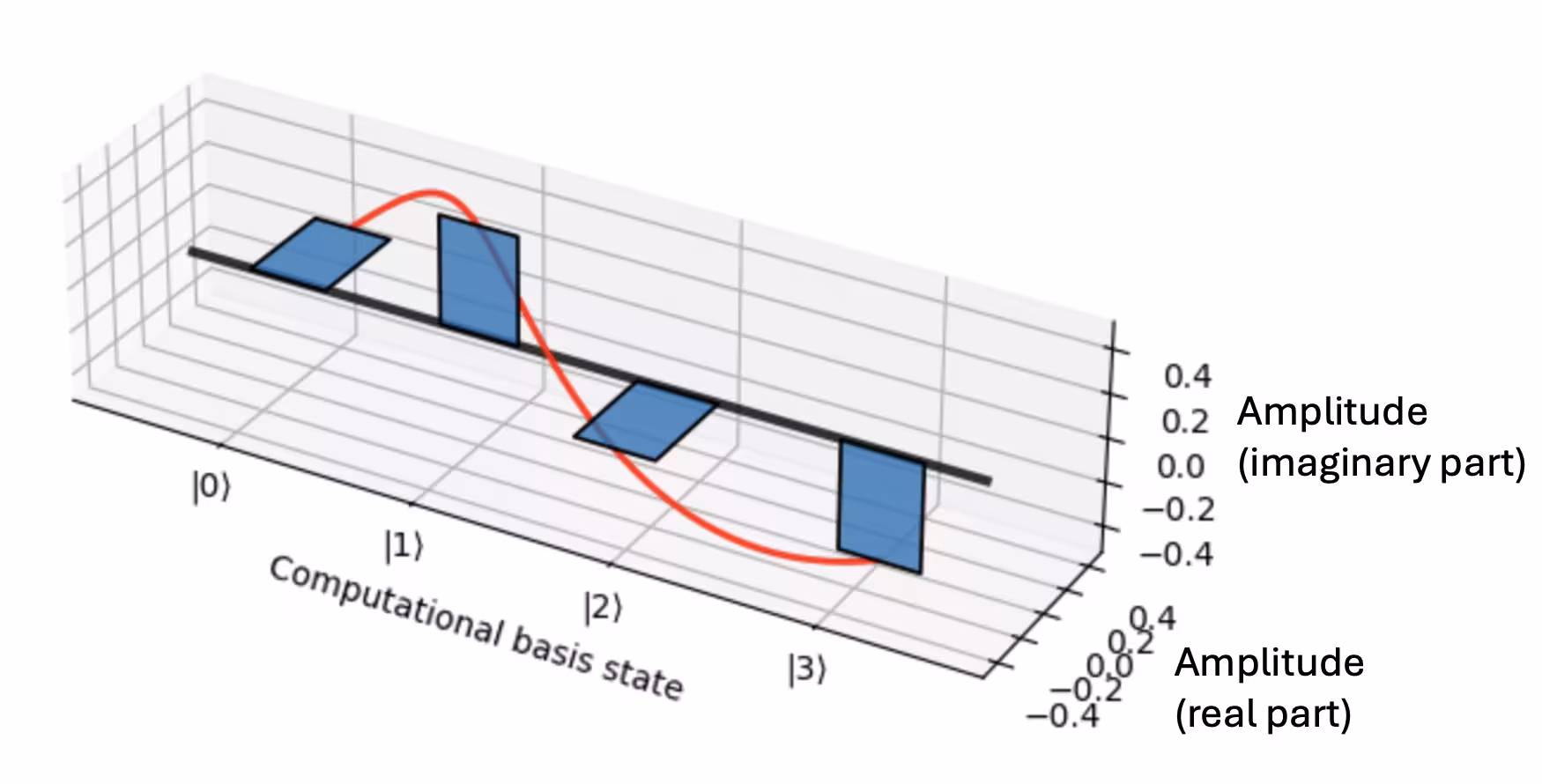
Ainsi, chaque état a une phase supérieure de $2\pi/4$ radians à l'état précédent lorsqu'ils sont ordonnés de la façon habituelle, car dans cet exemple on a quatre états de base ($N=4$). L'état de base suivant s'enroule de 0 à $2\pi$ deux fois :

$|\phi_2\rangle = \frac{1}{2} (|00\rangle + e^{i\pi}|01\rangle + e^{2i\pi}|10\rangle + e^{3i\pi}|11\rangle) = \frac{1}{2} (|00\rangle - |01\rangle + |10\rangle - |11\rangle)$

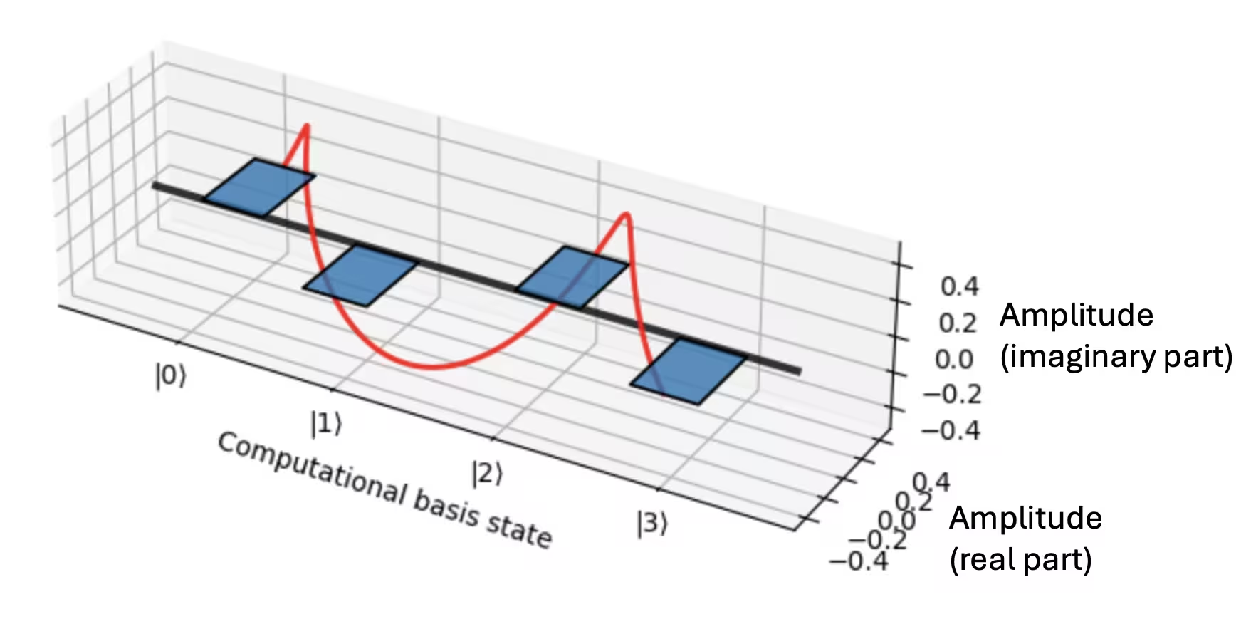
Enfin, la composante de Fourier la plus élevée est celle dont la phase varie le plus rapidement. Pour notre exemple avec deux qubits, c'est celle dont les phases s'enroulent de 0 à $2\pi$ trois fois :

$|\phi_3\rangle = \frac{1}{2} (|00\rangle + e^{3i\pi/2}|01\rangle + e^{6i\pi/2}|10\rangle + e^{9i\pi/2}|11\rangle) = \frac{1}{2} (|00\rangle - i|01\rangle - |10\rangle + i|11\rangle)$

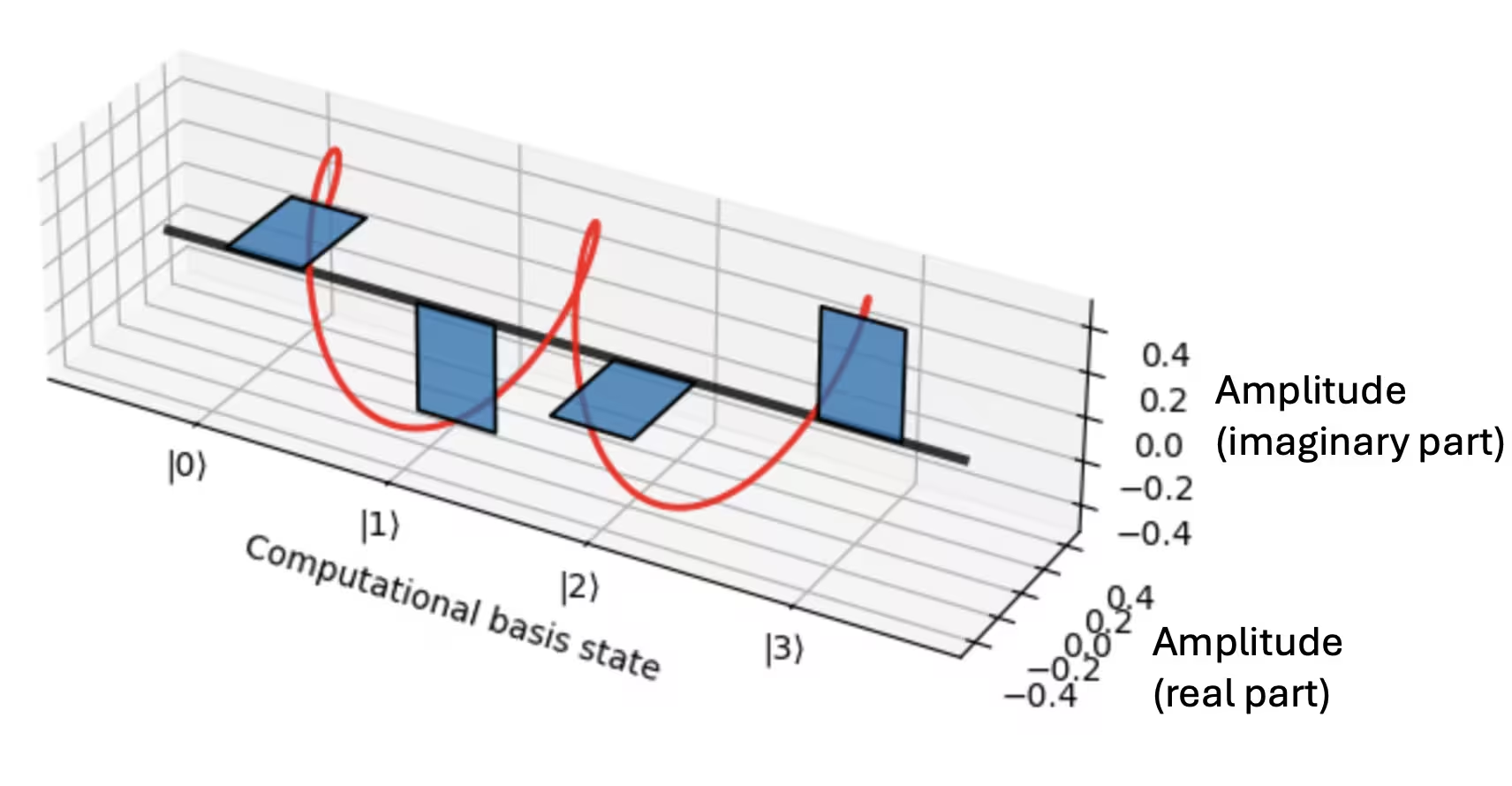
En général, pour un état à $m$ qubits, il y aura $2^m$ états de base de Fourier, dont la fréquence de variation de phase va de constante pour $|\phi_0\rangle$ à rapidement variable pour $|\phi_{2^m-1}\rangle$, complétant $2^m-1$ tours autour de $2\pi$ sur la superposition d'états. Donc, quand on applique une QFT à un état quantique, on fait essentiellement la même analyse de base qu'on a faite pour la forme d'onde musicale dans l'introduction. On détermine les composantes fréquentielles de Fourier qui contribuent à créer l'état quantique d'intérêt.

Essaie quelques exemples de QFT

Continuons à développer notre intuition pour la transformée de Fourier quantique en préparant un état dans la base computationnelle, puis en observant ce qui se passe lorsqu'on applique la QFT. Pour l'instant, on va traiter la QFT comme une boîte noire qu'on applique avec le QFTGate de la bibliothèque de circuits Qiskit. Plus tard, on regardera sous le capot pour voir comment elle est implémentée.

On commence par charger les packages nécessaires et sélectionner un dispositif pour exécuter notre circuit :

import numpy as np
from qiskit import QuantumCircuit
from qiskit.visualization import plot_histogram
from qiskit.circuit.library import QFTGate

# Load the Qiskit Runtime service
from qiskit_ibm_runtime import QiskitRuntimeService

# Load the Runtime primitive and session
from qiskit_ibm_runtime import SamplerV2 as Sampler

service = QiskitRuntimeService()

# Use the least busy backend
# backend = service.least_busy(operational=True, simulator=False, min_num_qubits = 127)
backend = service.backend("ibm_pinguino2")

print(backend.name)

ibm_pinguino2

Si tu n'as pas de temps disponible sur ton compte ou si tu veux utiliser un simulateur pour une raison quelconque, tu peux exécuter la cellule ci-dessous pour configurer un simulateur qui imitera le dispositif quantique qu'on a sélectionné ci-dessus :

# Load the backend sampler
from qiskit.primitives import BackendSamplerV2

# Load the Aer simulator and generate a noise model based on the currently-selected backend.
from qiskit_aer import AerSimulator
from qiskit_aer.noise import NoiseModel

noise_model = NoiseModel.from_backend(backend)

# Define a simulator using Aer, and use it in Sampler.
backend_sim = AerSimulator(noise_model=noise_model)
sampler_sim = BackendSamplerV2(backend=backend_sim)

# Alternatively, load a fake backend with generic properties and define a simulator.
from qiskit.providers.fake_provider import GenericBackendV2

backend_gen = GenericBackendV2(num_qubits=18)
sampler_gen = BackendSamplerV2(backend=backend_gen)

Un seul état de base computationnel

D'abord, essayons de transformer un seul état de base computationnel. On commence par créer un état computationnel aléatoire :

# Step 1: Map

qubits = 4
N = 2**qubits

qc = QuantumCircuit(qubits)

# flip state of random qubits to put in a random single computational basis state
for i in range(1, qubits):
    if np.random.randint(0, 2):
        qc.x(i)

# make a copy of the above circuit. (to be used when we apply the QFT in next part)
qc_qft = qc.copy()

qc.measure_all()
qc.draw("mpl")

# Step 2: Transpile
from qiskit.transpiler.preset_passmanagers import generate_preset_pass_manager

target = backend.target
pm = generate_preset_pass_manager(target=target, optimization_level=3)

qc_isa = pm.run(qc)

# Step 3: Run the job on a real quantum computer OR try fake backend

sampler = Sampler(mode=backend)
pubs = [qc_isa]

# Run the job on real quantum device

job = sampler.run(pubs, shots=1000)
res = job.result()
counts = res[0].data.meas.get_counts()

# OR Run the job on the Aer simulator with noise model from real backend

# job = sampler_sim.run([qc_isa])
# res = job.result()
# counts = res[0].data.meas.get_counts()

# Step 4: Post-Process
plot_histogram(counts)

Maintenant, appliquons la transformée de Fourier à cet état avec QFTGate :

# Step 1: Map

qc_qft.compose(QFTGate(qubits), inplace=True)
qc_qft.measure_all()
qc_qft.draw("mpl")

# Step 2: Transpile
from qiskit.transpiler.preset_passmanagers import generate_preset_pass_manager

target = backend.target
pm = generate_preset_pass_manager(target=target, optimization_level=3)

qc_isa = pm.run(qc_qft)

# Step 3: Run the job on a real quantum computer - try fake backend

sampler = Sampler(mode=backend)
pubs = [qc_isa]

# Run the job on real quantum device

job = sampler.run(pubs, shots=1000)
res = job.result()
counts = res[0].data.meas.get_counts()

# OR Run the job on the Aer simulator with noise model from real backend

# job = sampler_sim.run([qc_isa])
# res = job.result()
# counts = res[0].data.meas.get_counts()

# Step 4: Post-Process
plot_histogram(counts)

Comme tu peux le voir, on mesure les populations de chaque état comme étant plus ou moins égales, à quelques bruits expérimentaux et statistiques près. Donc, si on applique la QFT à un seul état de base computationnel, le résultat est une superposition égale de tous les états. Si tu es familier avec les transformées de Fourier, cela ne te surprend probablement pas. Un principe de base qui peut nous aider à construire une connexion intuitive entre une fonction et sa transformée de Fourier est que la largeur d'une fonction est inversement proportionnelle à la largeur de sa transformée de Fourier. Donc, quelque chose de très localisé dans le temps, par exemple une très courte impulsion, nécessitera une large gamme de fréquences pour générer cette impulsion. Ce signal sera très étendu dans l'espace de Fourier.

Ce fait est en réalité lié à l'incertitude quantique ! Le principe d'incertitude de Heisenberg est généralement énoncé comme $\Delta x \Delta p \ge \hbar / 2$. Donc si l'incertitude sur $x$ ($\Delta x$) est petite, l'incertitude sur la quantité de mouvement ($\Delta p$) doit être grande, et vice versa. Il s'avère que passer de la base de position $x$ à la base d'impulsion $p$ s'accomplit via une transformée de Fourier.

Note : Garde à l'esprit qu'on mesure les populations dans chacun des états de base, donc on perd des informations sur les phases relatives entre les différentes parties de la superposition. Ainsi, bien que la QFT de n'importe quel état de base computationnel unique donne la même répartition égale en population sur tous les états de base, les phases ne seront pas nécessairement les mêmes.

Deux états de base computationnels

Voyons maintenant ce qui se passe quand on prépare une superposition d'états de base computationnels. À ton avis, à quoi ressemblera la transformée de Fourier dans ce cas ?

Choisissons la superposition :

$|\psi\rangle = \frac{1}{\sqrt{2}} (|0\rangle + |N/2\rangle) = \frac{1}{\sqrt{2}} (|000...0\rangle + |100...0\rangle)$

# Step 1: Map
qubits = 4
N = 2**qubits

qc = QuantumCircuit(qubits)

# To make this state, we just need to apply a Hadamard to the last qubit

qc.h(qubits - 1)

qc_qft = qc.copy()

qc.measure_all()

qc.draw("mpl")

# First, let's go through steps 2-4 for the first circuit, qc

# Step 2: Transpile
from qiskit.transpiler.preset_passmanagers import generate_preset_pass_manager

target = backend.target
pm = generate_preset_pass_manager(target=target, optimization_level=3)

qc_isa = pm.run(qc)

# Step 3: Run the job on a real quantum computer - try fake backend

sampler = Sampler(mode=backend)
pubs = [qc_isa]

# Run the job on real quantum device

job = sampler.run(pubs, shots=1000)
res = job.result()
counts = res[0].data.meas.get_counts()

# OR run the job on the Aer simulator with noise model from real backend

# job = sampler_sim.run([qc_isa])
# res = job.result()
# counts = res[0].data.meas.get_counts()

# Step 4: Post-process
plot_histogram(counts)

Maintenant, appliquons la transformée de Fourier à cet état avec QFTGate :

# Step 1: Map

qc_qft.compose(QFTGate(qubits), inplace=True)
qc_qft.measure_all()
qc_qft.draw("mpl")

# Step 2: Transpile
from qiskit.transpiler.preset_passmanagers import generate_preset_pass_manager

target = backend.target
pm = generate_preset_pass_manager(target=target, optimization_level=3)

qc_isa = pm.run(qc_qft)

# Step 3: Run the job on a real quantum computer OR try fake backend

sampler = Sampler(mode=backend)
pubs = [qc_isa]

# Run the job on real quantum device

job = sampler.run(pubs, shots=1000)
res = job.result()
counts = res[0].data.meas.get_counts()

# OR run the job on the Aer simulator with noise model from real backend

# job = sampler_sim.run([qc_isa])
# res = job.result()
# counts = res[0].data.meas.get_counts()

# Step 4: Post-process
plot_histogram(counts)

Ce résultat pourrait être un peu surprenant. On dirait que la QFT de l'état $|\psi\rangle = \frac{1}{\sqrt{2}} (|0\rangle + |N/2\rangle)$ est une superposition de tous les états de base pairs. Mais si on repense à notre visualisation de chaque état de base $|\phi_y\rangle$, et à la façon dont la phase de chaque composante s'enroule $y$ fois autour de $2\pi$, la raison pour laquelle on obtient ce résultat devrait devenir claire.

Vérifie ta compréhension

Lis la ou les questions ci-dessous, réfléchis à ta réponse, puis clique sur le triangle pour révéler la solution.

En utilisant l'indice ci-dessus, explique pourquoi le résultat qu'on a obtenu pour la QFT de $|\psi\rangle = \frac{1}{\sqrt{2}} (|0\rangle + |N/2\rangle)$ est attendu.

Réponse :

L'état original a une phase relative de 0 (ou un multiple entier de $2\pi$) entre les deux parties de la superposition. On sait donc que cet état a des composantes de Fourier dont les phases s'accordent de cette façon : celles qui ont un déphasage nul entre le terme |0000> et le terme |1000>. Chaque état de base de Fourier $|\phi_y\rangle$ est composé de termes dont la phase s'accumule à un taux de $2\pi y/N$, ce qui signifie que, ordonnés de la façon habituelle, chaque terme de la superposition a une phase de $2\pi y/N$ supérieure au terme précédent. Donc, au point médian $N/2$, on veut que la phase $2\pi y/N * N/2$ soit un multiple entier de $2\pi$. Cela se produit quand $y$ est pair.

Quelle superposition d'états computationnels correspondrait à une QFT avec des pics sur chaque nombre binaire impair ?

Réponse :

Si tu appliquais la QFT à l'état $\psi = |0\rangle - |N/2\rangle$, tu verrais des pics sur chaque état numéroté binaire impair.

Décompose l'algorithme QFT

Maintenant qu'on a acquis plus d'intuition sur la relation entre les états de qubits dans la base computationnelle et la base de Fourier, creusons dans l'algorithme QFT lui-même. En d'autres termes, quelles portes applique-t-on réellement sur l'ordinateur quantique pour réaliser cette transformée ?

Commençons petit, avec un seul qubit. Ça signifie qu'on aura deux états de base. QFT$_2$ transforme les états de base computationnels $|0\rangle$ et $|1\rangle$ en états de base de Fourier $\phi_0$ et $\phi_1$ :

$|\phi_0\rangle = \frac{1}{\sqrt{2}}(|0\rangle + |1\rangle)$

$|\phi_1\rangle = \frac{1}{\sqrt{2}}(|0\rangle - |1\rangle)$

Vérifie ta compréhension

Lis la ou les questions ci-dessous, réfléchis à ta réponse, puis clique sur le triangle pour révéler la solution.

Utilise l'équation de la QFT de la section précédente pour vérifier ces deux états de base de Fourier ci-dessus.

Réponse :

La formule générale de la QFT est :

$| \phi_y \rangle = \frac{1}{\sqrt{N}}\sum_{x=0}^{N-1}\omega_N^{y x} \vert x \rangle$

Pour un seul qubit ($n=1$), $N=2^n=2$, et $\omega_N^{xy} = e^{2\pi i \frac {y x}{2}}$. Donc on a :

$| \phi_0 \rangle = \frac{1}{\sqrt{2}}(e^{2\pi i \frac {0 \times 0}{2}}|0\rangle + e^{2\pi i \frac {0 \times 1}{2}}|1\rangle) = \frac{1}{\sqrt{2}}(|0\rangle + |1\rangle)$

$| \phi_1 \rangle = \frac{1}{\sqrt{2}}(e^{2\pi i \frac {1 \times 0}{2}}|0\rangle + e^{2\pi i \frac {1 \times 1}{2}}|1\rangle) = \frac{1}{\sqrt{2}}(|0\rangle - |1\rangle)$

Regarde ces deux équations. Tu connais peut-être déjà une porte quantique qui peut être utilisée pour implémenter cette transformée. C'est-à-dire qu'il existe une porte qui transforme les états de base computationnels $|0\rangle$ et $|1\rangle$ vers les états de base de Fourier respectifs $|\phi_0\rangle$ et $|\phi_1\rangle$. C'est une porte de Hadamard ! Cela devient encore plus clair si on introduit une représentation matricielle de l'opération QFT$_N$ :

$\text{QFT}_N = \frac{1}{\sqrt{N}} \sum_{x=0}^{N-1} \sum_{y=0}^{N-1} \omega_N^{xy} \vert x \rangle \langle y \vert$

Si tu n'es pas familier avec cette notation pour exprimer un opérateur quantique, pas de problème ! C'est une façon de représenter une matrice $N \times N$, où $x$ et $y$ indexent les colonnes et les lignes de la matrice, de $0$ à $N-1$, et $\omega_N^{xy}$ est la valeur de cet élément particulier. Ainsi, l'élément dans la 0e colonne et la 2e ligne, par exemple, serait simplement $\omega_N^{0,2} = e^{2 \pi i \frac{0 \times 2}{N}} = 1$.

Dans cette représentation, chacun des états de base computationnels est associé à l'un des vecteurs de base :

$$\begin{pmatrix} 1 \\ 0 \\ \vdots \\ 0 \end{pmatrix}, |1\rangle = \begin{pmatrix} 0 \\ 1 \\ \vdots \\ 0 \end{pmatrix}, |N-1\rangle = \begin{pmatrix} 0 \\ 0 \\ \vdots \\ 1 \end{pmatrix}.$$

Si tu veux approfondir cette représentation, consulte la leçon de John Watrous sur les systèmes multiples dans le cours Bases de l'information quantique.

Essayons de construire la matrice pour QFT$_4$. En utilisant la formule ci-dessus, on trouve que :

\text\{QFT\}_4 = \frac\{1\}\{2\} \begin\{pmatrix\} 1 & 1 & 1 & 1 \\ 1 & i & -1 & -i \\ 1 & -1 & 1 & -1 \\ 1 & -i & -1 & i \\ \end\{pmatrix\}

Pour implémenter cette matrice sur un ordinateur quantique, on doit déterminer quelle combinaison de portes appliquées à quels qubits donnera une transformation unitaire qui correspond à la matrice ci-dessus. On sait déjà qu'une des portes nécessaires est la Hadamard. Une autre porte dont on aura besoin est la porte de phase contrôlée, qui applique une phase relative $\alpha$ à l'état du qubit cible, à condition que le qubit de contrôle soit dans l'état $|1\rangle$. En forme matricielle, cela ressemble à :

\text\{CP\}_\alpha = \begin\{pmatrix\} 1 & 0 & 0 & 0 \\ 0 & 1 & 0 & 0 \\ 0 & 0 & 1 & 0 \\ 0 & 0 & 0 & e^\{i\alpha\} \\ \end\{pmatrix\}

Comme seul l'état $|11\rangle$ est modifié, peu importe en fait quel qubit est considéré comme le « contrôle » et quel est la « cible ». Le résultat sera le même dans les deux cas.

Enfin, on aura aussi besoin de portes SWAP. Une porte SWAP échange les états de deux qubits. Elle ressemble à :

\text\{SWAP\}_\alpha = \begin\{pmatrix\} 1 & 0 & 0 & 0 \\ 0 & 0 & 1 & 0 \\ 0 & 1 & 0 & 0 \\ 0 & 0 & 0 & 1 \\ \end\{pmatrix\}

La procédure pour construire un circuit QFT$_{2^m}$ sur $m$ qubits est itérative — on applique d'abord QFT$_{2^{m-1}}$ aux qubits $1$ à $m-1$, puis on ajoute quelques portes entre le qubit $0$ et les $m-1$ autres qubits. Mais pour appliquer QFT$_{2^{m-1}}$, il faut d'abord appliquer QFT$_{2^{m-2}}$ aux qubits 2 à $m-1$, puis ajouter quelques portes entre le qubit 1 et les qubits restants $2$ à $m-1$. C'est comme une poupée russe : chaque poupée multiplie par deux la dimension du circuit QFT, la plus petite poupée étant au centre, qui est QFT$_2$, ou la porte de Hadamard.

Pour mettre une poupée à l'intérieur de la prochaine taille supérieure, augmentant ainsi la dimension de la QFT d'un facteur deux, on suit toujours la même procédure :

1. D'abord, applique QFT$_{2^{m-1}}$ aux $m-1$ qubits les plus bas. C'est ta « petite poupée » du jeu de poupées russes que tu vas bientôt mettre dans la poupée de taille suivante.
2. Utilise le qubit suivant vers le haut comme contrôle, et applique des portes de phase contrôlée à chacun des $m-1$ qubits du bas, avec des phases vers les états de base standard de chacun des $m-1$ qubits restants.
3. Effectue une Hadamard sur ce même qubit le plus haut qui a été utilisé comme contrôle dans les portes de phase.
4. Utilise des portes SWAP pour permuter l'ordre des qubits afin que le bit le moins significatif (haut) devienne le bit le plus significatif (bas), et que tous les autres remontent d'un.

On a déjà utilisé la fonction QFTGate de la bibliothèque de circuits Qiskit, mais regardons maintenant à l'intérieur de certaines de ces portes QFT pour vérifier la procédure ci-dessus. On peut le faire avec decompose().

qc = QuantumCircuit(1)
qc.compose(QFTGate(1), inplace=True)
qc.decompose().draw("mpl")

qc = QuantumCircuit(2)
qc.compose(QFTGate(2), inplace=True)
qc.decompose().draw("mpl")

qc = QuantumCircuit(3)
qc.compose(QFTGate(3), inplace=True)
qc.decompose().draw("mpl")

qc = QuantumCircuit(4)
qc.compose(QFTGate(4), inplace=True)
qc.decompose().draw("mpl")

Donc, en regardant les quatre premières QFT, tu devrais commencer à voir comment chacune est imbriquée dans la suivante. Tu as peut-être remarqué, cependant, que certaines des portes de phase ne sont pas exactement celles prescrites dans la procédure qu'on a décrite ci-dessus, et les SWAP n'apparaissent pas après chaque sous-routine, mais seulement à la toute fin de la QFT complète. Cela nous évite des portes inutiles, qui allongeraient le temps d'exécution du circuit et le rendraient plus sujet aux erreurs. Au lieu d'implémenter le SWAP après chaque poupée imbriquée, le circuit garde la trace de l'endroit où chaque état de qubit devrait se trouver et ajuste les qubits auxquels il applique les portes de phase en conséquence. Ensuite, un ensemble final de SWAP à la fin remet tout en place.

Applique la QFT : estimation de phase

Voyons comment la QFT peut être utilisée pour résoudre un problème utile en informatique quantique. Calculer la transformée de Fourier quantique inverse est une étape nécessaire dans un algorithme connu sous le nom d'Estimation de Phase Quantique (QPE), qui est elle-même une sous-routine dans de nombreux autres algorithmes, notamment le « joyau de la couronne » des algorithmes quantiques, l'algorithme de factorisation de Shor.

L'objectif de la QPE est d'estimer les valeurs propres d'un opérateur unitaire. Les opérateurs unitaires sont omniprésents en informatique quantique, et souvent, trouver les valeurs propres de leurs vecteurs propres associés est une étape nécessaire dans un algorithme plus large. Selon le problème, une valeur propre peut représenter une énergie d'un Hamiltonien dans un problème de simulation, peut nous aider à trouver les facteurs premiers d'un nombre dans l'algorithme de Shor, ou peut contenir d'autres informations essentielles. La QPE est l'une des sous-routines les plus importantes et les plus utilisées en informatique quantique.

Alors, quel rapport avec une transformée de Fourier quantique ? Eh bien, comme tu t'en souviens peut-être, toute valeur propre $\lambda$ d'un opérateur unitaire a un module $|\lambda| = 1$. On peut donc écrire chaque valeur propre comme un nombre complexe de module un :

$\lambda = e^{2\pi i \theta}$

où $\theta$ est un nombre réel entre 0 et 1. Si tu veux plus d'informations sur les matrices unitaires, consulte la leçon de John Watrous sur le sujet dans Bases de l'information quantique.

Note que $\lambda$ est périodique en $\theta$. Cela pourrait déjà te suggérer qu'une QFT pourrait être impliquée, puisqu'on a vu comment les QFT sont utiles pour analyser les fonctions périodiques. Ci-dessous, on va parcourir l'algorithme et voir précisément comment la QFT entre en jeu.

Comment fonctionne la QPE

D'abord, on va commencer par l'algorithme QPE le plus simple, qui estime grossièrement la phase à un seul chiffre binaire de précision. En d'autres termes, cet algorithme peut distinguer entre $\theta = 0$ et $\theta = 1/2$, mais ne peut pas faire mieux. Voici le schéma du circuit :

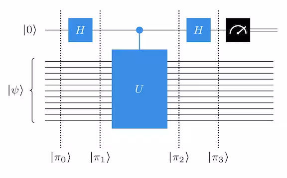
Les qubits sont préparés dans l'état $|\pi_0\rangle = |\psi\rangle|0\rangle$, où le qubit $0$ est dans l'état $|0\rangle$ et les qubits restants sont dans l'état $|\psi\rangle$, qui est un état propre de $U$. Après la première Hadamard, l'état des qubits devient :

$|\pi_1\rangle = \frac{1}{\sqrt{2}}|\psi\rangle (|0\rangle + |1\rangle)$

La porte suivante est une porte « U contrôlée ». Elle applique l'opération unitaire $U$ aux qubits du bas dans l'état $|\psi\rangle$ si le qubit 0 est dans l'état $|1\rangle$, mais ne fait rien à $|\psi\rangle$ si le qubit 0 est dans l'état $|0\rangle$. Cela transforme les qubits vers l'état :

$|\pi_2\rangle = \frac{1}{\sqrt{2}}( |\psi\rangle|0\rangle + e^{2\pi i \theta}|\psi\rangle|1\rangle)$ $= \frac{1}{\sqrt{2}}|\psi\rangle (|0\rangle + e^{2\pi i \theta}|1\rangle)$

Quelque chose d'étrange vient de se passer : la porte U contrôlée n'utilise le qubit $0$ que comme qubit de contrôle, donc on pourrait penser que cette porte ne changerait pas du tout l'état du qubit 0. Mais d'une façon ou d'une autre, c'est le cas ! Même si l'opération a été appliquée aux qubits inférieurs, l'effet global de la porte est de changer la phase du qubit $0$. C'est ce qu'on appelle le « mécanisme de rétroaction de phase » (phase kickback), et il est utilisé dans de nombreux algorithmes quantiques, notamment Deutsch-Josza et l'algorithme de Grover. Si tu veux en savoir plus sur le mécanisme de rétroaction de phase, consulte la leçon de John Watrous sur les algorithmes de requête quantique dans Fondamentaux des algorithmes quantiques.

Après la rétroaction de phase, on applique encore une Hadamard au qubit $0$, ce qui donne l'état :

$|\pi_3\rangle = |\psi\rangle ( \frac{1+e^{2\pi i \theta}}{2} |0\rangle + \frac{1 - e^{2\pi i \theta}}{2}|1\rangle) = |\psi\rangle ( \cos(\pi\theta) |0\rangle - i \sin(\pi\theta)|1\rangle)$

Donc, quand on mesure le qubit $0$ à la fin, on mesurera $|0\rangle$ avec une certitude de 100% si $\theta = 0$ et on mesurera $|1\rangle$ avec une certitude de 100% si $\theta = \frac{1}{2}$ (et si notre ordinateur quantique est parfait, sans bruit). Si $\theta$ est différent de ces valeurs, la mesure finale n'est que probabiliste et ne nous dit que peu de choses.

QPE avec plus de précision : plus de qubits

On peut étendre ce concept simple à un algorithme plus complexe avec une précision arbitraire. Si au lieu d'utiliser seulement le qubit $0$ pour mesurer la phase, on utilise $m$ qubits de $0$ à $m-1$, on pourra estimer la phase avec $m$ bits de précision. Voyons comment ça fonctionne :

Ce circuit QPE plus précis commence de la même façon que la version à un bit : des Hadamards sont appliquées aux $m$ premiers qubits, et les qubits restants sont préparés dans l'état $|\psi\rangle$, créant l'état :

$|\pi_1\rangle = \frac{1}{2^{m/2}}|\psi\rangle(|0\rangle+|1\rangle)(|0\rangle+|1\rangle)...(|0\rangle+|1\rangle)$

Maintenant, les unitaires contrôlées sont appliquées. Le qubit $0$ est le contrôle pour le même unitaire $U$ qu'avant. Mais maintenant, le qubit $1$ est le contrôle pour l'unitaire $U^2$, qui est simplement $U$ appliqué deux fois. Donc, la valeur propre de $U^2$ est $e^{2*2\pi i \theta}$. En général, chaque qubit $k$ de 0 à $m-1$ sera le contrôle pour l'unitaire $U^{2^k}$. Cela signifie que chacun de ces qubits subira une rétroaction de phase de $e^{2^k*2\pi i \theta}$. Cela donne l'état :

$|\pi_2\rangle = |\psi\rangle \otimes \frac{1}{2^{m/2}} (|0\rangle+e^{2^{m-1}2\pi i \theta}|1\rangle)(|0\rangle+e^{2^{m-2}2\pi i \theta}|1\rangle)...(|0\rangle+e^{2\pi i \theta}|1\rangle)$

Cela peut être réécrit comme une somme sur les états de base computationnels :

$|\pi_2\rangle = |\psi\rangle \otimes \frac{1}{2^{m/2}} \sum_{k=0}^{2^{m}-1} e^{2\pi i k \theta} |k\rangle$

La somme te semble familière ? C'est une QFT ! Rappelle-toi l'équation de la transformée de Fourier quantique :

$\text{QFT}_{2^m}| y \rangle = \frac{1}{\sqrt{2^m}}\sum_{x=0}^{2^m-1}\omega_{2^m}^{y x} \vert x \rangle$

Donc, si la phase $\theta = y/2^m$ pour un entier $y$ entre $0$ et $2^m-1$, alors appliquer la QFT inverse à cet état donnera l'état :

$|\pi_3\rangle = |\psi\rangle \otimes |y\rangle$

et à partir de $|y\rangle$, on peut déduire $\theta$.

Si $\theta/2^m$ n'est pas un multiple entier, en revanche, alors appliquer la QFT inverse ne fera qu'approximer $\theta$. La qualité de l'approximation de $\theta$ sera probabiliste, ce qui signifie qu'on n'obtiendra pas toujours la meilleure approximation, mais elle sera assez proche, et plus on utilise de qubits $m$, meilleure sera l'approximation. Pour apprendre à quantifier cette approximation de $\theta$, consulte la leçon de John Watrous sur l'estimation de phase et la factorisation dans Fondamentaux des algorithmes quantiques.

Conclusion

Ce module a donné un aperçu de ce qu'est une QFT, de la façon dont elle est implémentée sur un ordinateur quantique, et de son utilité pour résoudre des problèmes. On t'a donné un avant-goût de son utilité en voyant comment elle peut être utilisée dans l'estimation de phase quantique pour en apprendre davantage sur les valeurs propres d'une matrice unitaire.

Concepts clés

• La Transformée de Fourier Quantique est l'analogue quantique de la Transformée de Fourier Discrète.
• La QFT est un exemple de transformation de base.
• La procédure d'Estimation de Phase Quantique repose sur le mécanisme de rétroaction de phase des opérations unitaires contrôlées, ainsi que sur une QFT inverse.
• La QFT et la QPE sont toutes deux des sous-routines largement utilisées dans de nombreux algorithmes quantiques.

Questions

Vrai/Faux

1. V/F La Transformée de Fourier Quantique est l'analogue quantique de la transformée de Fourier discrète (DFT) classique.
2. V/F La QFT peut être implémentée en utilisant uniquement des portes de Hadamard et des portes CNOT.
3. V/F La QFT est un composant clé de l'algorithme de Shor.
4. V/F La sortie de l'Estimation de Phase Quantique est un état quantique représentant le vecteur propre de l'opérateur.
5. V/F La QPE nécessite l'utilisation de la Transformée de Fourier Quantique inverse (QFT$^\dag$).
6. V/F Dans la QPE, si la phase $\phi$ est exactement représentable avec $n$ bits, l'algorithme donne le résultat correct avec une probabilité 1.

Réponses courtes

1. Combien de qubits sont nécessaires pour effectuer une QFT sur un système avec $2^n$ points de données ?
2. La QFT peut-elle être utilisée sur un état qui n'est pas un état de base computationnel ? Si oui, que se passe-t-il ?
3. Comment le nombre de qubits de contrôle utilisés dans la QPE affecte-t-il la résolution de l'estimation de phase résultante ?

Problèmes

1. Utilise la multiplication matricielle pour vérifier que les étapes de l'algorithme QFT donnent bien la matrice $\text{QFT}_4$ :

$$\text{QFT}_4 = \frac{1}{2} \begin{pmatrix} 1 & 1 & 1 & 1 \\ 1 & i & -1 & -i \\ 1 & -1 & 1 & -1 \\ 1 & -i & -1 & i \\ \end{pmatrix}$$

(Tu n'as pas besoin de le faire à la main !)

Problèmes de défi

1. Crée un état à quatre qubits qui est une superposition égale de toutes les bases computationnelles impaires : $|\psi\rangle = |0001\rangle + |0011\rangle + |0101\rangle + |0111\rangle +|1001\rangle +|1011\rangle +|1101\rangle +|1111\rangle$. Ensuite, effectue une QFT sur l'état. Quel est l'état résultant ? Explique pourquoi ton résultat est cohérent, en utilisant tes connaissances des transformées de Fourier.