Annulation probabiliste des erreurs avec cônes de lumière ombrés
Estimation d'utilisation : 10 minutes sur un processeur Heron (REMARQUE : il s'agit uniquement d'une estimation. Ton temps d'exécution peut varier.)
Résultats d'apprentissage
-
Ce qu'est l'annulation probabiliste des erreurs (PEC), et pourquoi son surcoût d'échantillonnage croît de façon exponentielle avec le bruit total agissant sur le circuit
-
Comment les cônes de lumière ombrés (SLC) bornent la contribution de chaque terme de bruit à l'observable cible, afin de pouvoir dépenser le budget d'atténuation là où c'est important — et comment, au-delà de la réduction de surcoût à biais nul déjà fournie par un cône de lumière purement géométrique, l'ombrage permet d'échanger un biais résiduel borné contre un surcoût d'échantillonnage encore plus faible
-
Comment apprendre le bruit de couche avec
NoiseLearnerV3et injecter de l'anti-bruit viasamplomaticet la primitiveExecutor -
Comment combiner PEC et PEC+SLC avec TREX et la post-sélection pour estimer une valeur d'espérance sur du matériel
Prérequis
-
Le flux de travail des modèles Qiskit
-
L'utilisation de la primitive Estimator pour calculer les valeurs d'espérance d'une observable
-
Les techniques d'atténuation d'erreurs telles que le twirling de Pauli et TREX, abordées dans Combiner des options d'atténuation d'erreurs avec la primitive Estimator
Contexte
Ce tutoriel montre comment atténuer les erreurs en utilisant l'addon des cônes de lumière ombrés (SLC). Cet addon est une évolution de la technique d'annulation probabiliste des erreurs (PEC), dans laquelle un utilisateur apprend le bruit de couches uniques dans un circuit puis annule le bruit en appliquant des portes à un qubit et des techniques de post-traitement. Comparée à d'autres méthodes, la PEC offre des bornes plus robustes sur le biais du résultat atténué, mais tend à souffrir d'un surcoût plus élevé en temps QPU. Pendant la PEC, pour compenser l'atténuation de la valeur d'espérance par le bruit, le résultat moyen est remis à l'échelle par un facteur , où est le taux de bruit appris de l'erreur de Pauli à la couche du circuit. Cette remise à l'échelle augmente la variance d'un facteur , et multiplie donc également par le nombre d'exécutions de circuit nécessaires sur le QPU, ce que nous appelons le coût ou surcoût d'échantillonnage. Comme croît de façon exponentielle, la PEC est souvent limitée à des circuits peu profonds ou comportant peu de qubits. Pour en savoir plus sur la PEC, voir Annulation probabiliste des erreurs avec des modèles de Pauli-Lindblad épars sur des processeurs quantiques bruités.
Si nous pouvons identifier les erreurs qui n'ont pas besoin d'être atténuées, nous pouvons réduire ce coût d'échantillonnage de façon exponentielle. Une première étape dans cette direction consiste à mettre en œuvre une atténuation d'erreurs à sensibilité locale, qui utilise un « cône de lumière » conventionnel rapidement calculable pour réduire le surcoût de la PEC en bornant la sensibilité d'une observable aux erreurs dans l'ensemble du circuit, étendant la faisabilité de la PEC à de plus grandes échelles pour certains problèmes. Les erreurs situées en dehors de ce cône de lumière ne peuvent pas affecter le résultat mesuré et peuvent donc être exclues de la procédure d'annulation des erreurs. Cette exclusion diminue le surcoût d'échantillonnage, parfois de façon substantielle, sans introduire de biais supplémentaire. En particulier, pour la mesure d'une observable locale d'un circuit à profondeur fixe, le surcoût d'échantillonnage requis finit par atteindre un plateau lorsque le nombre de qubits du circuit augmente (voir Fig. 2b dans Localité et atténuation d'erreurs des circuits quantiques).
Les cônes de lumière ombrés (SLC) vont plus loin, en utilisant des simulations classiques pour borner plus étroitement la sensibilité aux erreurs dans l'ensemble du circuit. Cela échange du temps QPU contre du temps CPU et réduit le surcoût d'échantillonnage nécessaire pour renormaliser le biais. Au lieu d'une coupure nette, chaque erreur potentielle du circuit se voit attribuer une « ombre » graduée qui borne supérieurement la sensibilité de la valeur d'espérance de l'observable à cette erreur. (Pour les bornes propagées vers l'arrière introduites ci-dessous, cette sensibilité dépend aussi de l'état initial du circuit — l'état tout-zéro dans les flux de travail typiques, et dans ce tutoriel.) Cette caractérisation affinée permet des applications plus efficaces et ciblées de la PEC avec une variance réduite, tout en donnant à l'utilisateur la capacité d'ajuster de manière contrôlée le biais dans l'estimation de l'observable. Voir Ombrage des cônes de lumière pour l'atténuation d'erreurs quantiques accélérée classiquement pour plus de détails.
Notre flux de travail pour l'addon SLC s'appuie sur la bibliothèque samplomatic ainsi que sur les classes QuantumProgram et Executor ajoutées à Qiskit Runtime dans qiskit-ibm-runtime v0.47.0, permettant aux utilisateurs d'avoir un contrôle plus modulaire des paramètres d'exécution pour la suppression et l'atténuation des erreurs tout en conservant une facilité d'utilisation. Pour en savoir plus, consulte le guide sur le modèle d'exécution dirigée.
Vue d'ensemble du flux de travail d'atténuation d'erreurs SLC
Pour modéliser le bruit du QPU, nous utilisons un modèle de bruit de Pauli-Lindblad épars avec des taux d'erreur de Pauli à un et deux qubits, générés localement sur chaque qubit et chaque arête de l'appareil. Avec ce choix, le flux de travail d'atténuation d'erreurs SLC présenté dans ce tutoriel est le suivant :
a. CPU — Borner l'impact par erreur des erreurs de Pauli à un et deux qubits
-
Propagation vers l'avant (borne de l'effet sur l'observable). Propager chaque erreur jusqu'à la fin du circuit et calculer son commutateur avec l'observable.
-
Tronquer les termes d'opérateur pendant l'évolution afin de garder le calcul faisable.
-
Resserrer encore ces bornes par une propagation arrière lâche de l'observable basée sur les limites de vitesse quantique.
-
-
Propagation vers l'arrière (borne de l'effet sur l'état initial). Propager chaque erreur jusqu'au début du circuit et calculer son commutateur avec l'état initial.
b. QPU — Apprendre les taux de bruit. Utiliser NoiseLearnerV3 pour estimer les taux du modèle de bruit de Pauli-Lindblad.
c. CPU — Prioriser l'atténuation
-
Mettre à jour les bornes fusionnées avec les taux de bruit appris. Combiner les bornes avant et arrière précédemment calculées et les mettre à jour avec les taux de bruit appris.
-
Classer les composantes de bruit à atténuer en utilisant les bornes calculées et les taux appris. Prioriser chaque erreur de bruit possible en fonction de son impact estimé sur le biais et du coût associé pour la corriger.
d. QPU — Insérer l'anti-bruit et exécuter. Exécuter le circuit d'intérêt avec l'anti-bruit (bruit inverse) spécifié à l'aide d'annotations Box.
e. CPU — Estimer l'observable. Calculer la valeur d'espérance, en appliquant une post-sélection basée sur les mesures pour réduire l'impact du bruit non markovien.
Vue d'ensemble de l'apprentissage du bruit
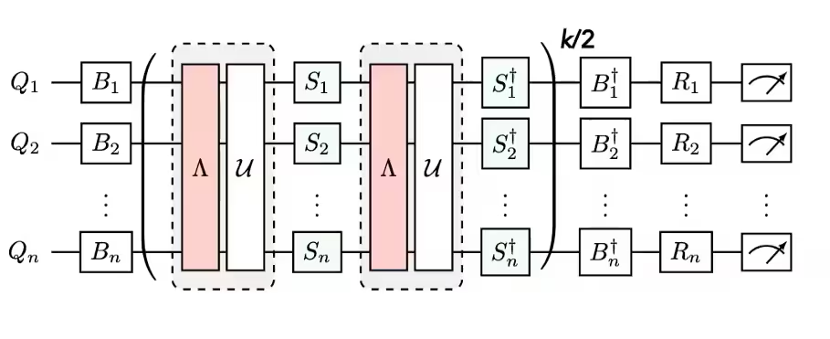
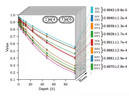
L'apprentissage du bruit est une étape courante dans plusieurs méthodes d'atténuation d'erreurs, réalisée par le module d'apprentissage du bruit ; il apparaît aussi dans le tutoriel sur l'amplification probabiliste des erreurs. Dans NoiseLearnerV3, tu peux identifier spécifiquement les couches de bruit à apprendre sous forme d'objets CircuitInstruction, afin de pouvoir calculer les bornes de bruit SLC souhaitées pour chaque couche de la manière décrite ci-dessus. Le modèle de Pauli-Lindblad appris fournit des coefficients à utiliser dans la priorisation PEC+SLC. La façon dont les portes sont regroupées en couches peut être déterminée à l'aide des fonctions utilitaires generate_boxing_pass_manager et find_unique_box_instructions, puis transmise à la fonction utilitaire SLC generate_noise_model_paulis, comme décrit à l'étape 2 ci-dessous.
| Partie 1 | Partie 2 | Partie 3 |
|---|---|---|
| Twirling de Pauli des couches de portes à deux qubits | Répéter des paires de couches identité et apprendre le bruit | Déduire une fidélité (erreur pour chaque canal de bruit) |
 |  |  |
Vue d'ensemble du post-traitement
Après l'exécution sur du matériel quantique en utilisant le cadre samplomatic et Executor, nous convertissons nos mesures de chaînes de bits en la valeur d'observable souhaitée. Dans ce tutoriel, nous montrons le flux de travail sur un circuit d'Ising en miroir (construit à l'étape 1 ci-dessous), pour lequel la valeur d'espérance idéale de l'observable mesurée est 1 car la seconde moitié du circuit annule la première. Lors du calcul de la valeur de l'observable avec la fonction executor_expectation_values, nous appliquons quelques techniques de post-traitement qui réduisent l'impact du bruit. Celles-ci comprennent la suppression des shots affectés par du bruit non markovien, l'atténuation des erreurs de lecture, et la prise en compte des détails de notre implémentation de la PEC. Les détails sont abordés à l'étape 4 ci-dessous.
Prérequis
Avant de commencer ce tutoriel, assure-toi d'avoir installé ce qui suit :
-
Qiskit SDK v2.2 ou ultérieur, avec le support de visualisation
-
Qiskit Runtime v0.47 ou ultérieur (
pip install qiskit-ibm-runtime) -
Addon Qiskit des cônes de lumière ombrés v0.1 ou ultérieur (
pip install qiskit-addon-slc) -
Addon utils Qiskit v0.3 ou ultérieur (
pip install qiskit-addon-utils) -
Samplomatic v0.13 ou ultérieur (
pip install samplomatic)
Configuration
Tout d'abord, importe les paquets et fonctions nécessaires à l'exécution de ce notebook.
# Added by doQumentation — required packages for this notebook
!pip install -q matplotlib numpy qiskit qiskit-addon-slc qiskit-addon-utils qiskit-ibm-runtime samplomatic
from multiprocessing import set_start_method

# Setting this value prevents itertools.starmap deadlock on UNIX systems
set_start_method("spawn")

# Needed to prevent PySCF from parallelizing internally (SLC only)
%set_env OMP_NUM_THREADS=1
env: OMP_NUM_THREADS=1
import numpy as np
from matplotlib import pyplot as plt

from qiskit import QuantumCircuit
from qiskit.quantum_info import SparsePauliOp
from qiskit.transpiler import generate_preset_pass_manager, PassManager

from qiskit_ibm_runtime import (
    QiskitRuntimeService,
    QuantumProgram,
    Executor,
    NoiseLearnerV3,
)

import samplomatic
from samplomatic.utils import find_unique_box_instructions
from samplomatic.transpiler import generate_boxing_pass_manager

from qiskit_addon_utils.exp_vals.measurement_bases import (
    get_measurement_bases,
)
from qiskit_addon_utils.exp_vals.expectation_values import (
    executor_expectation_values,
)
from qiskit_addon_utils.noise_management import (
    gamma_from_noisy_boxes,
    trex_factors,
)
from qiskit_addon_utils.noise_management.post_selection import PostSelector
from qiskit_addon_utils.noise_management.post_selection.transpiler.passes import (
    AddPostSelectionMeasures,
    AddSpectatorMeasures,
)

from qiskit_addon_slc.bounds import (
    compute_backward_bounds,
    compute_forward_bounds,
    compute_local_scales,
    merge_bounds,
    tighten_with_speed_limit,
)
from qiskit_addon_slc.utils import (
    generate_noise_model_paulis,
    map_modifier_ref_to_ref,
)
from qiskit_addon_slc.visualization import draw_shaded_lightcone
Exemple de simulateur à petite échelle
Comme d'autres méthodes d'atténuation d'erreurs basées sur l'apprentissage, la PEC avec cônes de lumière ombrés atténue le bruit physique d'un processeur quantique spécifique, elle dépend donc de services matériels sans analogue significatif sur un simulateur idéal :
-
NoiseLearnerV3caractérise expérimentalement le canal de bruit de Pauli-Lindblad épars sur chaque couche unique à deux qubits. Sur un simulateur sans bruit, il n'y a pas de bruit à annuler. -
La primitive
Executoréchantillonne les circuits twirlés, injectés d'anti-bruit, générés parsamplomaticsur un backend.
Le calcul de la borne du cône de lumière ombré est classique, mais il n'a de sens que par rapport aux taux de bruit matériel appris, qui déterminent le budget d'atténuation et le surcoût d'échantillonnage. Pour ces raisons, nous sautons l'exemple de simulateur à petite échelle et démontrons directement le flux de travail complet PEC+SLC sur du matériel, avec chaque étape du modèle Qiskit détaillée ci-dessous.
Exemple matériel à grande échelle
Nous exécutons le flux de travail PEC+SLC complet sur un circuit d'Ising en miroir à 20 qubits exécuté sur du matériel IBM Quantum®, en suivant les quatre étapes d'un modèle Qiskit.
Étape 1 : Représenter le problème
Notre démonstration est configurée comme suit :
-
Nous choisissons d'effectuer une évolution temporelle sous un hamiltonien de chaîne d'Ising 1D. La chaîne d'Ising 1D donne une structure de circuit agréablement dense, ce qui est pratique pour illustrer des implémentations de PEC.
-
Nous choisissons de mesurer l'observable , qui contient une composante et une composante . Cela est pratique pour mettre en évidence comment les bornes SLC traitent différemment les différents types d'erreurs.
-
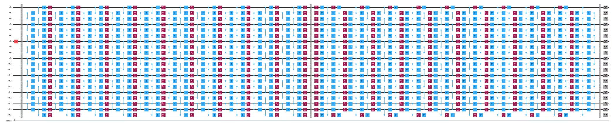
Nous voulons que la valeur d'espérance idéale de cette observable soit exactement 1, afin que la qualité des estimations atténuées soit facile à juger. La mise en miroir du circuit nous fait faire la majeure partie du chemin : pour chaque porte dans la seconde moitié du circuit, il existe une porte inverse dans la première moitié, de sorte que le circuit idéal agisse comme l'identité.
-
Enfin, pour obtenir la valeur d'espérance idéale de 1, il faut que le circuit commence — et donc, grâce à la mise en miroir, se termine idéalement aussi — dans un état propre +1 de l'observable. Étant donné que l'observable contient une composante non-, et que la primitive
Executorprend en compte la base de mesure souhaitée à la fin du circuit, nous ajoutons les portes de préparation de base correspondantes au début du circuit miroir avec une fonctionprepare_basis. Nous utilisons la fonctionget_measurement_basespour identifier quelles portes sont nécessaires et où les placer, tout en suivant les subtilités d'index de qubit issues des conventions d'annotationbox, comme discuté dans la section sur la préparation des mesures de base canoniques.
# Width of the Ising chain (a free parameter of this demonstration)
num_qubits = 20

# The observable to measure: one X component (on qubit 6) and one Z component
# (on qubit 13), as motivated in "Step 1: Map the problem" above
target_obs_sparse = [("XZ", [6, 13], 1.0)]
observable = SparsePauliOp.from_sparse_list(
    target_obs_sparse, num_qubits=num_qubits
)
# Determine the measurement basis each qubit requires for this observable.
# The reverser is used during post-processing in Step 4.
bases_virt, reverser_virt = get_measurement_bases(observable)
# Free parameters of the demonstration circuit: the number of Trotter steps
# sets the circuit depth, and rx_angle is the transverse-field rotation angle
# applied in each step (pi/4 makes the dynamics non-Clifford)
num_trotter_steps = 10
rx_angle = np.pi / 4
def construct_ising_circuit(
    num_qubits: int,
    num_trotter_steps: int,
    rx_angle: float,
) -> QuantumCircuit:
    circuit = QuantumCircuit(num_qubits)

    for _ in range(num_trotter_steps):
        circuit.rx(rx_angle, range(num_qubits))
        for first_qubit in (1, 2):
            for idx in range(first_qubit, num_qubits, 2):
                # equivalent to Rzz(-pi/2):
                circuit.sdg([idx - 1, idx])
                circuit.cz(idx - 1, idx)

    return circuit

def prepare_basis(
    circuit: QuantumCircuit, basis: list[int]
) -> QuantumCircuit:
    # basis is a list of integer values from 0 to 3. These map to the basis measurement as:
    # 0 = I; 1 = Z; 2 = X; 3 = Y
    assert len(basis) == circuit.num_qubits

    out_circ = circuit.copy_empty_like()
    for qb, bas in enumerate(basis):
        if bas == 2:
            out_circ.h(qb)
        elif bas == 3:
            out_circ.rx(-np.pi / 2, qb)

    out_circ.barrier()
    out_circ.compose(circuit, inplace=True)
    return out_circ

def mirror_circuit(circuit: QuantumCircuit) -> QuantumCircuit:
    mirror_circ = circuit.copy_empty_like()
    mirror_circ.compose(circuit.inverse(), inplace=True)
    mirror_circ.barrier()
    mirror_circ.compose(circuit, inplace=True)
    mirror_circ.measure_active()
    return mirror_circ
# Instantiate the mirrored circuit and prepend the basis-preparation gates
circuit = construct_ising_circuit(num_qubits, num_trotter_steps, rx_angle)
mirrored_circuit = mirror_circuit(circuit)
mirrored_circuit = prepare_basis(mirrored_circuit, bases_virt[0])
mirrored_circuit.draw(
    "mpl", fold=-1, scale=0.3, idle_wires=False, measure_arrows=False
)
Étape 2 : Optimiser
Nous optimisons les détails associés au circuit à exécuter, à l'observable à mesurer, et aux paramètres d'apprentissage du bruit. Comme point de départ, nous sélectionnons le processeur Heron le moins occupé et l'instancions avec les portes fractionnaires activées. Ces portes fractionnaires permettent une plus grande sensibilité dans certains de nos filtres de post-sélection.
# Initialize IBM Quantum Compute Service using your saved credentials
service = QiskitRuntimeService()

# Select the least busy Heron device. This tutorial targets Heron processors:
# the usage estimate and the non-Markovian-noise post-selection discussed in
# Step 4 are specific to this processor family.
backend = service.least_busy(
    operational=True,
    simulator=False,
    filters=lambda b: b.processor_type["family"] == "Heron",
)
# Re-fetch with fractional gates enabled (least_busy does not forward this)
# Fractional gates are enabled so the non-Clifford Rx rotations are supported natively.
backend = service.backend(backend.name, use_fractional_gates=True)
print(f"Selected backend: {backend.name}")
Selected backend: ibm_kingston
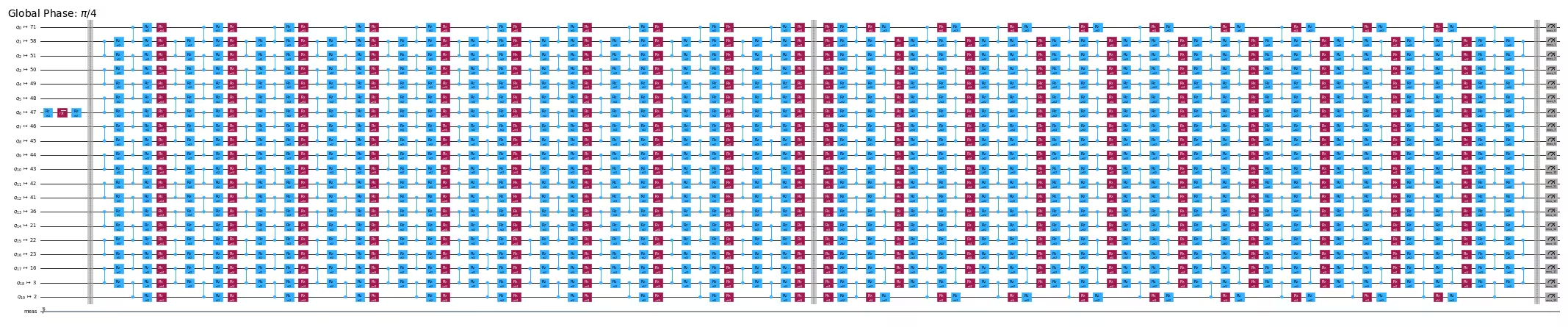
Tout d'abord, nous allons transpiler notre circuit en instructions ISA, comme requis pour l'exécution sur nos QPU. Le choix des qubits physiques sur lesquels s'exécuter a un impact important sur la qualité des résultats, car les temps de cohérence et les fidélités des portes varient d'un appareil à l'autre et dérivent dans le temps. Pour une expérience soignée, il peut être payant de sélectionner manuellement une chaîne de qubits en s'appuyant sur des expériences de benchmarking rapides (voir, par exemple, le tutoriel Benchmarking en temps réel pour la sélection de qubits). Pour les besoins de ce tutoriel, nous nous appuyons sur le transpileur Qiskit pour sélectionner une disposition basée sur la carte de couplage du backend et ses données de calibration les plus récentes.
isa_pm = generate_preset_pass_manager(backend=backend, optimization_level=1)

isa_circuit = isa_pm.run(mirrored_circuit)

# The chain of physical qubits selected by the transpiler
layout = isa_circuit.layout.final_index_layout()
print(f"Selected layout: {layout}")

isa_observable = observable.apply_layout(
    layout, num_qubits=isa_circuit.num_qubits
)
Selected layout: [71, 58, 51, 50, 49, 48, 47, 46, 45, 44, 43, 42, 41, 36, 21, 22, 23, 16, 3, 2]
wire_order = layout + [
    q for q in range(isa_circuit.num_qubits) if q not in layout
]
isa_circuit.draw(
    "mpl",
    fold=-1,
    scale=0.3,
    idle_wires=False,
    wire_order=wire_order,
    measure_arrows=False,
)
Encadrer le circuit (box)
Pour faciliter l'implémentation, nous utilisons la passe de transpilation generate_boxing_pass_manager, qui place les instructions du circuit dans des boîtes annotées. Ces boîtes indiquent clairement où, dans le cas de PEC, l'anti-bruit doit être injecté dans le circuit. Pour plus de détails sur les paramètres, consultez la documentation Samplomatic.
Notez que le workflow SLC nécessite l'utilisation de inject_noise_strategy="individual_modification" plus tard dans le processus, car cela nous permet d'identifier de manière unique les annotations InjectNoise des instructions BoxOp dans le circuit. (Les boîtes sans annotation InjectNoise ne peuvent pas être identifiées de cette manière.)
Les calculs de bornes SLC supposent actuellement que les annotations InjectNoise sont placées avec site="after" (voir qiskit-addon-slc#33). Comme la valeur par défaut de ce paramètre a changé dans les versions récentes de samplomatic (voir samplomatic#372), nous définissons explicitement inject_noise_site="after" ci-dessous.
La fonction find_unique_box_instructions parcourt le circuit encadré fourni et identifie ceux qui ont des couches à deux qubits (2Q) ou des mesures uniques, dans le but de l'apprentissage du bruit et de l'injection de bruit.
# Box circuit with Twirl and InjectNoise annotations
boxes_pm = generate_boxing_pass_manager(
    twirling_strategy="active",
    inject_noise_strategy="individual_modification",
    inject_noise_site="after",
    inject_noise_targets="gates",
    measure_annotations="all",
)

boxed_circuit = boxes_pm.run(isa_circuit)

# Find the unique instructions (layers) from boxed circuit
unique_2q_instructions = find_unique_box_instructions(
    boxed_circuit, normalize_annotations=None, undress_boxes=True
)
boxed_circuit.draw(
    "mpl",
    fold=-1,
    scale=0.3,
    idle_wires=False,
    wire_order=wire_order,
    measure_arrows=False,
)

Préparer les mesures de base canoniques
Notez que nous devons prendre un soin particulier à suivre l'ordre des qubits. Ci-dessous, nous introduisons la notion de canonical_qubits comme moyen de mettre à jour de manière appropriée l'ordre des qubits lors de sa fourniture à Executor, en raison de la façon dont l'ordre des qubits est capturé lors de l'encadrement des circuits et de la recherche des instructions uniques. Voir la documentation Convention d'ordre des qubits pour plus de détails.
# Determine the canonical qubits order
meas_box = boxed_circuit.data[-1]
canonical_qubits = [
    idx
    for idx, qubit in enumerate(boxed_circuit.qubits)
    if qubit in meas_box.qubits
]

# map canonical qubit to physical (isa) qubit
c_2_p = {c: p for c, p in enumerate(canonical_qubits)}
# map physical (isa) qubit to virtual qubit (index in original circuit)
p_2_v = {p: v for v, p in enumerate(layout)}
# compute map between virtual and canonical qubit indices.
c_2_v = {c: p_2_v[p] for c, p in c_2_p.items()}

assert len(c_2_v) == num_qubits

bases_canon = [
    np.array([base_i[c_2_v[c]] for c in range(num_qubits)], dtype=np.uint8)
    for base_i in bases_virt
]
Workflow pour l'ombrage de cône de lumière, l'apprentissage du bruit et l'injection d'anti-bruit
Dans ce tutoriel, nous exécutons les calculs de bornes SLC avant que l'apprentissage du bruit ne soit terminé, de sorte que le circuit à atténuer soit exécuté aussi près que possible dans le temps du modèle de bruit appris. En principe, ce workflow peut être encore parallélisé : un job d'apprentissage du bruit peut s'exécuter pendant que, en parallèle, les bornes de bruit sont estimées. Pour un circuit quantique arbitraire, le calcul des bornes de bruit peut évoluer avec une dépendance faiblement exponentielle, donc paralléliser le calcul des bornes (par exemple, sur plusieurs cœurs de CPU) produit des bornes plus serrées pour un budget de temps de calcul donné, et les exécutions QPU et les calculs de bornes peuvent eux-mêmes être parallélisés pour le workflow le plus efficace.
Prédire les Pauli du modèle de bruit à apprendre
Avant d'exécuter tout apprentissage du bruit sur le matériel, nous énumérons d'abord quels termes d'erreur de Pauli notre modèle de bruit contiendra. Rappelons que nous modélisons le bruit de chaque couche unique comme un modèle de Pauli-Lindblad épars avec un taux d'erreur pour chaque Pauli de poids un (, ou ) sur chaque qubit actif, et un pour chaque Pauli de poids deux sur chaque paire connectée de qubits actifs. La fonction generate_noise_model_paulis parcourt chaque couche encadrée unique du circuit fourni et génère exactement cette liste de termes de Pauli, en tenant compte de la connectivité des qubits du circuit.
En d'autres termes, cette étape prédit la structure du modèle de bruit que NoiseLearnerV3 remplira plus tard avec les taux appris. Connaître cette structure à l'avance est ce qui nous permet de calculer une borne avant et une borne arrière pour chaque erreur potentielle avant même que l'apprentissage du bruit n'ait été exécuté.
noise_model_paulis = generate_noise_model_paulis(
    unique_2q_instructions, backend.coupling_map, boxed_circuit
)
noise_model_rates = {ref: None for ref in noise_model_paulis}
a. Calculer les bornes avant
La fonction compute_forward_bounds évalue les relations de commutation entre les portes de chaque couche et les termes de Pauli générés ci-dessus, en termes de la façon dont les erreurs de propagation avant affectent l'observable souhaitée . Pour les portes qui commutent avec les termes de Pauli, rien n'est fait. Pour les portes de Clifford, elles sont poussées vers le début du circuit. Pour les portes non-Clifford, nous approximons leur influence sur les observables cibles pour être ultérieurement priorisées pour l'annulation du bruit (après que toutes les bornes ont été fusionnées). Cette borne est obtenue en appliquant d'abord la norme L2 (à savoir, la racine carrée de la somme des carrés des coefficients des termes de Pauli pertinents). Lorsqu'il y a trop de termes de qubits impliqués, nous revenons à une borne plus lâche qui utilise l'inégalité triangulaire.
Définir les paramètres de calcul des bornes
Les paramètres suivants contrôlent les calculs de bornes classiques :
-
slc_atol: la tolérance absolue des calculs. Les termes d'opérateur avec des coefficients inférieurs à ce seuil sont traités comme négligeables et écartés. -
slc_eigval_max_qubits: le nombre maximal de qubits pour lequel la borne plus stricte, basée sur les valeurs propres (norme L2), est évaluée. Les opérateurs pris en charge sur plus de qubits que cela reviennent à la borne plus lâche par inégalité triangulaire décrite ci-dessus. -
slc_evolution_max_terms: le nombre maximal de termes de Pauli conservés lors de la propagation des opérateurs à travers le circuit. La troncature des plus petits termes permet de garder le calcul gérable au prix de bornes légèrement plus lâches. -
slc_num_processes: le nombre de processus CPU sur lesquels le calcul des bornes est parallélisé. -
slc_timeout: le budget de temps (en secondes) pour le calcul des bornes. Toute couche non atteinte dans ce budget se voit attribuer la borne triviale de 2.
Dans ce tutoriel, le délai d'attente est atteint délibérément : nous gardons slc_timeout volontairement petit afin que le notebook s'exécute rapidement, et pour démontrer que l'atteinte du délai d'attente est sans danger. Les nuances calculées sont des bornes supérieures à chaque étape, donc atteindre le délai d'attente ne fait que rendre les bornes plus lâches (trivial) pour les couches qui n'ont pas été atteintes ; cela ne sous-estime jamais l'effet d'une erreur. Cela apparaît dans les visualisations ci-dessous comme les couches les plus à gauche étant entièrement remplies avec la borne triviale. Augmenter le délai d'attente (ou le nombre de processus) resserre les bornes et réduit davantage la surcharge d'échantillonnage.
slc_atol = 1e-8
slc_eigval_max_qubits = 18
slc_evolution_max_terms = 1000
slc_num_processes = 8
slc_timeout = 60
forward_bounds = compute_forward_bounds(
    boxed_circuit,
    noise_model_paulis,
    isa_observable,
    evolution_max_terms=slc_evolution_max_terms,
    eigval_max_qubits=slc_eigval_max_qubits,
    atol=slc_atol,
    num_processes=slc_num_processes,
    timeout=slc_timeout,
)
Bounds computation timed out.
Visualiser le SLC pour une inspection manuelle
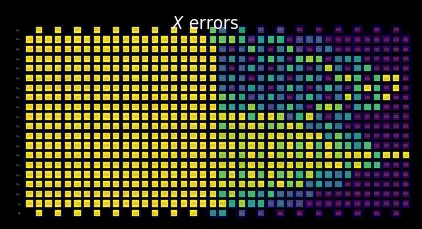
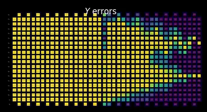
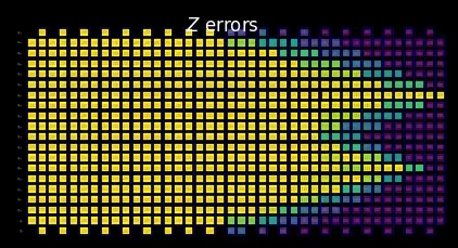
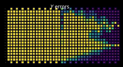
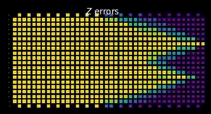
Vous pouvez interpréter le comportement des bornes ombrées en examinant comment les mesures et les termes de Pauli interagissent avec les erreurs locales. Ces motifs sont caractéristiques de ce problème d'évolution temporelle du hamiltonien d'Ising à impulsion (kicked Ising) et apparaissent également dans l'article Lightcone Shading for Classically Accelerated Quantum Error Mitigation, avec plusieurs caractéristiques révélatrices :
-
Nous pouvons clairement distinguer les deux cônes provenant des deux Paulis non-identité dans l'observable.
-
Nous pouvons voir que la mesure X sur le qubit 6 commute avec l'erreur X dans la couche la plus à droite.
-
Nous pouvons voir que le Pauli Z sur le qubit 13 commute avec l'erreur Z dans la couche la plus à droite.
-
Lorsque nous atteignons le délai spécifié ci-dessus, les couches restantes à gauche sont entièrement remplies de bornes triviales de deux.
for p in "XYZ":
    display(
        draw_shaded_lightcone(
            boxed_circuit,
            forward_bounds,
            noise_model_paulis,
            pauli_filter=p,
            scale=0.15,
            fold=-1,
            idle_wires=False,
            wire_order=wire_order,
            measure_arrows=False,
        )
    )
b. Resserrer les bornes avant avec les limites de vitesse quantique
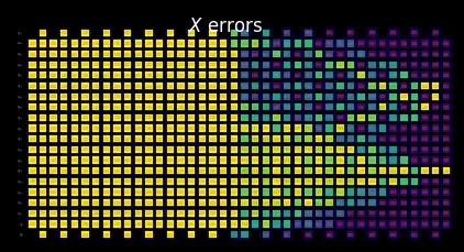
Nous resserrons ensuite les bornes en utilisant la fonction tighten_with_speed_limit. La propagation géométrique du cône de lumière de l'observable est déjà entièrement prise en compte dans les bornes avant calculées ci-dessus. Ce que cette fonction ajoute est une passe d'auto-cohérence qui exploite la vitesse limitée à laquelle l'information peut circuler à travers le circuit — le cône de lumière croît d'au plus un qubit par couche de portes à deux qubits — pour resserrer les bornes précédemment calculées les unes par rapport aux autres. L'information circule dans les deux directions :
-
Des bornes de commutateur aux bornes sur l'observable rétropropagée : si l'observable commute avec une erreur sur un qubit, alors elle ne peut pas avoir beaucoup de composante ou à cet endroit.
-
Des bornes sur l'observable rétropropagée aux bornes de commutateur : si l'observable a peu de composante et sur un qubit, alors elle doit presque commuter avec à cet endroit.
forward_bounds_tighter = tighten_with_speed_limit(
    forward_bounds, boxed_circuit, noise_model_paulis, isa_observable
)
Visualiser le SLC pour une inspection manuelle
En principe, ce resserrement fournit une transition plus douce entre les bornes calculées et les bornes triviales attribuées aux couches au-delà du délai. Dans cet exemple, l'effet est à peine visible, car les cônes de lumière se sont déjà propagés jusqu'aux bords du circuit au moment où le délai est atteint.
for p in "XYZ":
    display(
        draw_shaded_lightcone(
            boxed_circuit,
            forward_bounds_tighter,
            noise_model_paulis,
            pauli_filter=p,
            scale=0.15,
            fold=-1,
            idle_wires=False,
            wire_order=wire_order,
            measure_arrows=False,
        )
    )
c. Calculer les bornes arrière
Cette partie de la prédiction du bruit évalue comment une erreur à une couche particulière peut affecter l'état d'entrée . La fonction compute_backward_bounds inverse d'abord le circuit et supprime les portes de mesure, puis procède à une analyse similaire à celle effectuée pour les calculs des bornes avant.
backward_bounds = compute_backward_bounds(
    boxed_circuit,
    noise_model_paulis,
    evolution_max_terms=slc_evolution_max_terms,
    num_processes=slc_num_processes,
    timeout=slc_timeout,
)
Visualiser le SLC pour une inspection manuelle
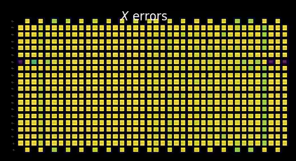
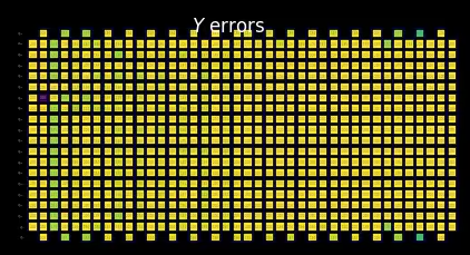
À partir du calcul des bornes arrière, nous pouvons voir comment la structure de l'état initial gouverne le comportement précoce de la propagation des erreurs :
-
Nous pouvons clairement voir comment les erreurs Z commutent initialement avec l'état initial |0⟩.
-
Seulement sur le qubit 6, où nous initialisons l'état propre +1 de la base X, une erreur Z ne parvient pas à commuter, tandis qu'une erreur X commute.
for p in "XYZ":
    display(
        draw_shaded_lightcone(
            boxed_circuit,
            backward_bounds,
            noise_model_paulis,
            pauli_filter=p,
            scale=0.15,
            fold=-1,
            idle_wires=False,
            wire_order=wire_order,
            measure_arrows=False,
        )
    )
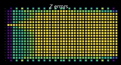
Aperçu des bornes fusionnées sans les taux de bruit appris
La fonction merged_bounds détermine le point dans le circuit où le passage des bornes arrière aux bornes avant minimise le biais total estimé sur l'observable souhaitée. Ce biais est calculé comme la somme des contributions des bornes arrière pour tous les emplacements de bruit avant ce point, plus les contributions des bornes avant pour tous les emplacements de bruit après celui-ci. Actuellement, cela est fait de manière uniforme pour tous les qubits.
Le point optimal auquel passer des bornes arrière aux bornes avant dépend des taux de bruit appris. À ce stade, nous n'avons encore appris aucun taux : noise_model_rates a été initialisé à None pour chaque couche, ce que merge_bounds traite comme des taux de bruit uniformes. Les bornes fusionnées présentées ici ne sont donc qu'un aperçu ; nous les recalculons avec les taux réellement appris à l'étape 3.
merged_bounds = merge_bounds(
    boxed_circuit,
    forward_bounds_tighter,
    backward_bounds,
    noise_model_rates,
)
Missing noise rates. Partitioning backward/forward commutator bounds by assuming uniform error rates.
Optimal spacetime partitioning not implemented!Just partitioning list of noisy boxes.
Visualiser le SLC pour une inspection manuelle
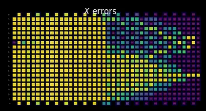
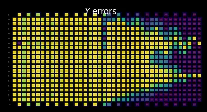
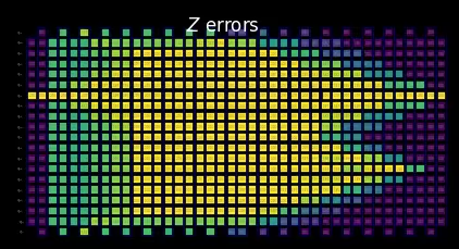
Après avoir fusionné les bornes arrière et les bornes avant resserrées, le comportement des SLC combinés devient clair :
-
La fonction ci-dessus nous indique qu'une partition est choisie à laquelle le passage des bornes arrière aux bornes avant resserrées a lieu.
-
Nous pouvons voir ci-dessous que les SLC contiennent maintenant des bornes arrière partielles et des bornes avant resserrées partielles.
for p in "XYZ":
    display(
        draw_shaded_lightcone(
            boxed_circuit,
            merged_bounds,
            noise_model_paulis,
            pauli_filter=p,
            scale=0.15,
            fold=-1,
            idle_wires=False,
            wire_order=wire_order,
            measure_arrows=False,
        )
    )
Étape 3 : Exécuter
Dans cette section, nous commençons la partie du workflow qui utilise un véritable dispositif quantique. Pour cette méthode d'atténuation d'erreur basée sur l'apprentissage, il y a deux étapes :
-
Apprendre le bruit en utilisant
NoiseLearnerV3. -
Exécuter un circuit d'atténuation d'erreur avec le framework
samplomaticetExecutor.
Avec les erreurs bornées de notre circuit quantique, nous apprenons les taux de bruit associés pour prioriser notre budget d'erreur, déterminer le surcoût d'échantillonnage, et exécuter sur un QPU.
a. Apprendre les taux de bruit
Le noise learner caractérise les processus de bruit affectant les portes dans un ou plusieurs circuits d'intérêt, en se basant sur le modèle de bruit de Pauli-Lindblad épars. La méthode run() lance une tâche d'apprentissage du bruit pour les couches à deux qubits uniques fournies, en utilisant les options spécifiées dans la configuration du noise learner. Ces options contrôlent la stratégie de twirling de Pauli, le nombre de randomisations et de shots, les profondeurs d'apprentissage, et la post-sélection.
Nous choisissons également les profondeurs d'apprentissage délibérément. Une constatation pratique pour l'atténuation basée sur l'apprentissage avec samplomatic est qu'il est très bénéfique que la profondeur d'apprentissage la plus profonde corresponde à la profondeur du circuit que vous souhaitez atténuer. Comme les layer_pair_depths de NLv3 sont mesurées en paires de couches (une couche plus son inverse), nous fixons la valeur la plus profonde à la moitié de la profondeur de couche à deux qubits du circuit.
post_selection_enabled = True
# Match the deepest noise-learning depth to the depth of the circuit being
# mitigated. NLv3 ``layer_pair_depths`` are measured in layer pairs (a layer
# plus its inverse), so the deepest value is half the circuit's two-qubit-layer
# depth. Learning to this depth markedly improves the quality of the mitigation.
#
# We measure the two-qubit-layer depth on the pre-boxed ISA circuit: after
# boxing, every two-qubit gate is hidden inside a full-width ``BoxOp``, so a
# ``num_qubits == 2`` filter on ``boxed_circuit`` matches nothing (and
# ``QuantumCircuit.depth`` does not recurse into boxes).
depth_2q = isa_circuit.depth(lambda instr: instr.operation.num_qubits == 2)
max_layer_pair_depth = depth_2q // 2  # dividing by 2 since we want pairs

# Use a fixed schedule of learning depths, but drop any that exceed the circuit's
# depth and always cap the deepest value at ``max_layer_pair_depth`` so we never
# learn deeper than the circuit being mitigated.
candidate_depths = [1, 2, 4, 8, 12, 16, 24, 32, 40, 48]
layer_pair_depths = sorted(
    {d for d in candidate_depths if d < max_layer_pair_depth}
    | {max_layer_pair_depth}
)

noise_learner_options = {
    "num_randomizations": 64,
    "shots_per_randomization": 128,
    "layer_pair_depths": layer_pair_depths,
    "post_selection": {
        "enable": post_selection_enabled,
        "strategy": "edge",
        "x_pulse_type": "rx",
    },
    "environment": {"job_tags": ["TUT_SLC"]},
}

noise_learner = NoiseLearnerV3(backend, noise_learner_options)
noise_learner_job = noise_learner.run(unique_2q_instructions)
noise_learner_result = noise_learner_job.result()
if post_selection_enabled:
    print(
        "Minimum fraction of shots kept for noise learning experiments: ",
        end="",
    )
    print(
        f"{min([min(d.values()) for d in [nlr.metadata['post_selection']['fraction_kept'] for nlr in noise_learner_result[:2]]]):.2f}"
    )
Minimum fraction of shots kept for noise learning experiments: 0.71
# Get a dict mapping each InjectNoise.ref to its learned PauliLindbladMap
refs_2_plm = noise_learner_result.to_dict(
    unique_2q_instructions, require_refs=False
)
b.i. Mettre à jour les bornes fusionnées avec les taux de bruit réellement appris
Maintenant que le modèle de bruit spécifique a été appris, nous pouvons appliquer les taux de bruit appris aux bornes de bruit prédites et obtenir une détermination finale des bornes qui ont le plus d'impact sur la minimisation du biais.
merged_bounds = merge_bounds(
    boxed_circuit,
    forward_bounds_tighter,
    backward_bounds,
    refs_2_plm,
)
Optimal spacetime partitioning not implemented!Just partitioning list of noisy boxes.
b.ii. Calculer les local_scales pour l'exécution matérielle
compute_local_scales examine chaque erreur de bruit possible dans le circuit et estime dans quelle mesure cette erreur pourrait biaiser la mesure finale, ainsi que le coût qu'il y aurait à la corriger. Elle classe ensuite les erreurs selon leur intérêt à être atténuées et sélectionne le sous-ensemble qui réduit le biais autant que possible, tout en restant dans le budget de coût d'échantillonnage autorisé (ou en atteignant une précision souhaitée). Le résultat est un ensemble de facteurs d'échelle indiquant quelles erreurs seront activement atténuées et lesquelles resteront non atténuées (local_scales), ainsi que le surcoût total d'échantillonnage prédit (sampling_costs) et le biais restant (residual_bias_bound).
La capacité à contrôler le biais restant souhaité est une fonctionnalité essentielle de l'implémentation SLC du PEC. Alors que dans l'implémentation originale, le surcoût d'échantillonnage visait toujours un biais nul, nous pouvons ajuster le surcoût d'échantillonnage requis avec un compromis sur le biais restant attendu. Cela aide l'utilisateur à rester dans un budget d'échantillonnage fixe, ce qui peut être particulièrement utile lors du prototypage initial d'un workflow.
id_map = map_modifier_ref_to_ref(boxed_circuit)
summed_rates = 0.0
for box_id, noise_id in id_map.items():
    learned_plm = refs_2_plm[noise_id]
    summed_rates += np.sum(learned_plm.rates)
    # print(f"{box_id}:\tgamma = {np.exp(2 * summed_rates):1.6e}\tsampling cost = {np.exp(4 * summed_rates):1.6e}")
total_gamma = np.exp(2 * summed_rates)
print(
    f"Full PEC gamma={total_gamma}, sampling cost (gamma^2) = {total_gamma**2}"
)
Full PEC gamma=12.750876317157042, sampling cost (gamma^2) = 162.58484685543633
biases = []
costs = []
for bias in [0.0] + np.arange(0.001, 0.102, 0.01).tolist():
    _, cost_, bias_ = compute_local_scales(
        boxed_circuit,
        merged_bounds,
        refs_2_plm,
        sampling_cost_budget=np.inf,
        bias_tolerance=bias,
    )
    biases.append(bias_)
    costs.append(cost_)
Faire un compromis entre le surcoût d'échantillonnage et le biais résiduel
xticks = np.arange(0, 11)

fig, ax = plt.subplots()
ax.scatter(
    [0], [total_gamma**2], marker="D", c="tab:orange", label="full PEC"
)
ax.plot(
    100 * np.array(biases),
    np.array(costs),
    "o-",
    c="tab:blue",
    label="PEC+SLC",
)
ax.set_yscale("log")
ax.set_xticks(xticks, [f"{x:.1f}" for x in xticks])

ax.set_xlabel("Remaining bias [%]")
ax.set_ylabel(r"Sampling overhead, $\gamma^2$")
ax.grid()
ax.legend()
fig.suptitle("PEC sampling overhead reduction due to SLC")
Text(0.5, 0.98, 'PEC sampling overhead reduction due to SLC')

chosen_bias_thres = 0.1
local_scales, sampling_cost, residual_bias_bound = compute_local_scales(
    boxed_circuit,
    merged_bounds,
    refs_2_plm,
    sampling_cost_budget=np.inf,
    bias_tolerance=chosen_bias_thres,
)
print(
    f"PEC+SLC sampling cost (gamma^2) = {sampling_cost} "
    f"w/ remaining bias = {100 * residual_bias_bound:.1f}%"
)
PEC+SLC sampling cost (gamma^2) = 48.13646509622307 w/ remaining bias = 10.0%
c. Exécuter le circuit d'intérêt avec l'anti-bruit
c.i. Préparer le circuit modèle en utilisant samplex
Le samplex est une sortie de la méthode build de Samplomatic, qui encode toutes les informations nécessaires pour générer des paramètres randomisés pour template_circuit. Ceux-ci sont ensuite utilisés pour configurer les objets QuantumProgram, qui sont à leur tour exécutés sur un QPU avec la primitive Executor. Chaque QuantumProgram peut contenir plusieurs éléments, que vous pouvez considérer comme une paire de template et samplex.
Consultez le tutoriel Hello samplomatic pour plus de détails.
# Build template circuit and samplex for later use with the "Executor"
template_circuit, samplex = samplomatic.build(boxed_circuit)
# Set up postselection if it's been enabled
if post_selection_enabled:
    # Set up post selection PM (to add PS instructions)
    post_selection_pm = PassManager(
        [
            AddSpectatorMeasures(backend.coupling_map),
            AddPostSelectionMeasures(x_pulse_type="rx"),
        ]
    )
    final_template_circuit = post_selection_pm.run(template_circuit)
else:
    final_template_circuit = template_circuit
c.ii. Configurer le QuantumProgram
num_randomizations = 4096
shots_per_randomization = 64
chunk_size = 256
# Set up QuantumProgram
program = QuantumProgram(shots=shots_per_randomization, noise_maps=refs_2_plm)

# no EM

# Collect up a dict of the other arguments that need to be bound to samplex_inputs
samplex_inputs = {
    f"noise_scales.{ref}": float(0) for ref in local_scales.keys()
}
samplex_inputs |= {"basis_changes": {"basis0": bases_canon[0]}}

# Convert samplex_inputs into a dict to pass to QuantumProgram
samplex_arguments = (
    samplex.inputs().bind(**samplex_inputs).make_broadcastable()
)

program.append_samplex_item(
    circuit=final_template_circuit,
    samplex=samplex,
    samplex_arguments=samplex_arguments,
    shape=(num_randomizations,),
    chunk_size=chunk_size,
)

# plain PEC

# Collect a dict of the other arguments that need to be bound to samplex_inputs
samplex_inputs = {
    f"noise_scales.{ref}": float(-1) for ref in local_scales.keys()
}
samplex_inputs |= {"basis_changes": {"basis0": bases_canon[0]}}

# Convert samplex_inputs into a dict to pass to QuantumProgram
samplex_arguments = (
    samplex.inputs().bind(**samplex_inputs).make_broadcastable()
)

program.append_samplex_item(
    circuit=final_template_circuit,
    samplex=samplex,
    samplex_arguments=samplex_arguments,
    shape=(num_randomizations,),
    chunk_size=chunk_size,
)

# PEC+SLC

# Collect a dict of the other arguments that need to be bound to samplex_inputs
samplex_inputs = {
    f"noise_scales.{ref}": float(-1) for ref in local_scales.keys()
}
samplex_inputs |= {"basis_changes": {"basis0": bases_canon[0]}}
samplex_inputs |= {"local_scales": local_scales}

# Convert samplex_inputs into a dict to pass to QuantumProgram
samplex_arguments = (
    samplex.inputs().bind(**samplex_inputs).make_broadcastable()
)

program.append_samplex_item(
    circuit=final_template_circuit,
    samplex=samplex,
    samplex_arguments=samplex_arguments,
    shape=(num_randomizations,),
    chunk_size=chunk_size,
)
c.iii. Exécuter le programme avec la primitive Executor
executor = Executor(backend)
job_exec = executor.run(program)
results_exec = job_exec.result()
Étape 4 : Post-traiter
Alors que nous calculons la valeur d'espérance finale d'intérêt en utilisant executor_expectation_values, nous mettons en œuvre quelques techniques de post-traitement pour aider à garantir que nous obtenons les résultats de la meilleure qualité possible. Tout d'abord, nous appliquons notre extinction d'erreur de lecture par twirling (TREX), qui prend en compte toute erreur survenant pendant le processus de lecture. Ensuite, nous corrigeons les erreurs dues au bruit non markovien sur nos backends Heron en utilisant une méthode de post-sélection. Cette méthode mesure les qubits actifs et spectateurs, puis applique une rotation lente à chaque qubit, puis mesure à nouveau. Dans les cas où les deux mesures ne confirment pas un qubit basculé comme prévu, ces shots sont écartés en appliquant un mask du PostSelector. Dans le calcul du masque, une stratégie spécifique peut être définie pour filtrer en fonction des nœuds à un seul qubit ou des arêtes de qubits spectateurs voisins, ce qui peut influencer à la fois le nombre de shots filtrés et la qualité des résultats.
measurement_noise_map = noise_learner_result[2].to_pauli_lindblad_map()
trex_scale_factors = trex_factors(measurement_noise_map, reverser_virt)
post_selection_strategy = "node"
def post_process_conv(datum, steps=16, gamma=None, ps=False, trex=False):
    meas = datum["meas"]
    flips = datum["measurement_flips.meas"]
    signs = datum.get("pauli_signs", None)

    meas_basis_axis = None
    avg_axis = 0

    mask = None
    if ps and post_selection_enabled:
        # Post-select the results
        post_selector = PostSelector.from_circuit(
            circuit=final_template_circuit, coupling_map=backend.coupling_map
        )

        # Compute the ps mask for filtering results
        mask = post_selector.compute_mask(
            datum, strategy=post_selection_strategy
        )

        # Compute fraction of shots kept from post selection
        total_num_shots = num_randomizations * shots_per_randomization
        ps_ratio = np.sum(mask) * 100 / total_num_shots / len(bases_canon)
        print(
            f"With {post_selection_strategy}-based post selection ({ps_ratio:.1f}% of shots kept):"
        )

    results = []
    for i in range(steps, num_randomizations + 1, steps):
        # Compute mitigated expvals w/out post-selection
        res = executor_expectation_values(
            meas[:i],
            reverser_virt,
            meas_basis_axis,
            avg_axis=avg_axis,
            measurement_flips=flips[:i],
            pauli_signs=signs[:i] if signs is not None else None,
            postselect_mask=mask[:i] if mask is not None else None,
            rescale_factors=trex_scale_factors if trex else None,
            gamma_factor=gamma,
        )
        results.append(res[0])
    return results
gamma_pec = gamma_from_noisy_boxes(refs_2_plm, id_map)
gamma_slc = gamma_from_noisy_boxes(refs_2_plm, id_map, local_scales)
steps = 16
results = {}

for label, result_idx, gamma, use_ps, use_trex in [
    ("PEC", 1, gamma_pec, True, True),
    ("PEC+SLC", 2, gamma_slc, True, True),
    ("Unmitigated", 0, None, False, False),
]:
    res = post_process_conv(
        results_exec[result_idx],
        steps=steps,
        gamma=gamma,
        ps=use_ps,
        trex=use_trex,
    )
    results[label] = res
With node-based post selection (24.1% of shots kept):
With node-based post selection (24.2% of shots kept):
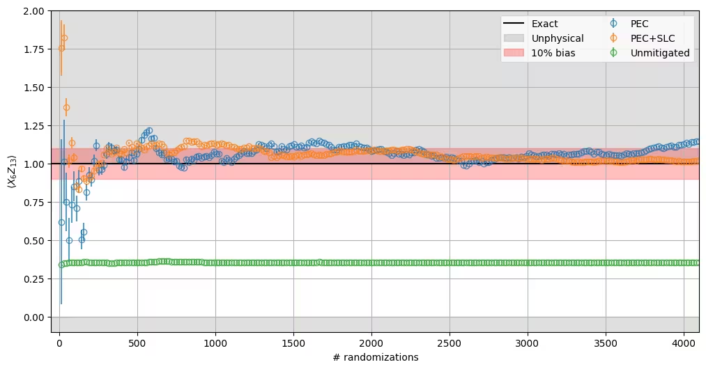
À partir de l'examen des résultats expérimentaux, nous pouvons directement comparer le comportement des différentes approches : PEC, PEC combiné avec SLC, et la référence non atténuée. Quelques détails spécifiques à souligner :
-
Le résultat non atténué se situe loin en dehors de la bande de biais de 10 % (proche de 0,35) et n'est pas affecté par le nombre de randomisations.
-
Sur cet appareil, le PEC complet entraîne un surcoût d'échantillonnage de . Après de fortes variations initiales, l'estimation du PEC simple récupère le signal et se stabilise autour de 1,1, dépassant légèrement la valeur exacte. Notez que la bande de biais de 10 % s'applique uniquement à l'estimateur PEC+SLC : le PEC simple est en principe non biaisé, donc cet écart résiduel n'est pas couvert par une garantie de biais mais reflète plutôt des fluctuations statistiques et des imperfections dans le modèle de bruit appris, ce qui est raisonnable à cette taille de problème.
-
Le SLC réduit encore le surcoût d'environ 3,4 fois (à , pour une borne de biais résiduel d'environ 10 %). Le PEC+SLC fluctue également fortement avec peu de randomisations, atteignant même initialement la région non physique, mais son estimation converge régulièrement vers la valeur exacte, se stabilisant près de 1,0 bien à l'intérieur de la bande. Il égale ou dépasse la précision du PEC simple pour environ un tiers du coût d'échantillonnage, démontrant l'avantage de l'ombrage de cône de lumière.
-
Les barres d'erreur des deux estimations atténuées se contractent à mesure que les randomisations s'accumulent ; à un nombre fixe de randomisations, l'estimateur PEC+SLC a la plus petite variance statistique, ce qui est cohérent avec son plus petit.
Notez que les taux de bruit appris (et donc les surcoûts et les estimations atténuées) dépendent du backend et de sa calibration au moment de l'exécution, de sorte que réexécuter ce notebook peut produire des valeurs quantitativement différentes.
fig, ax = plt.subplots(1, 1, figsize=(12, 6))

ax.axhline(1.0, color="black", label="Exact")
ax.fill_between(
    [-50, 4100], -10, 0, color="grey", alpha=0.25, label="Unphysical"
)
ax.fill_between([-50, 4100], 1, 10, color="grey", alpha=0.25)
ax.fill_between(
    [-50, 4100], 0.9, 1.1, color="red", alpha=0.25, label="10% bias"
)

for label, res in results.items():
    ax.errorbar(
        list(range(steps, num_randomizations + 1, steps)),
        [r[0] for r in res],
        yerr=[r[1] for r in res],
        alpha=0.75,
        marker="o",
        linestyle="",
        markerfacecolor="none",
        label=label,
    )

ax.set_ylabel(r"$\langle X_{6}Z_{13}\rangle$")
ax.set_xlabel("# randomizations")
ax.grid()

ax.legend(ncols=2)
ax.set_ylim([-0.1, 2.0])
ax.set_xlim([-50, 4100])
(-50.0, 4100.0)
Prochaines étapes
Si vous avez trouvé ce travail intéressant, vous pourriez être intéressé par les documents suivants :