Diagonalisation quantique de Krylov

Dans cette leçon sur la diagonalisation quantique de Krylov (DQK), nous répondrons aux questions suivantes :

• Qu'est-ce que la méthode de Krylov, en général ?
• Pourquoi la méthode de Krylov fonctionne-t-elle et dans quelles conditions ?
• Quel rôle joue l'informatique quantique dans ce contexte ?

La partie quantique des calculs est largement basée sur les travaux de la Réf. [1].

La vidéo ci-dessous donne un aperçu des méthodes de Krylov en informatique classique, en motive l'utilisation, et explique comment l'informatique quantique peut s'y intégrer. Le texte qui suit propose plus de détails et implémente une méthode de Krylov à la fois de façon classique et sur un ordinateur quantique.

1. Introduction aux méthodes de Krylov

Une méthode de sous-espace de Krylov peut désigner l'une des nombreuses méthodes construites autour de ce qu'on appelle le sous-espace de Krylov. Un tour d'horizon complet de ces méthodes dépasse le cadre de cette leçon, mais les Réf. [2-4] offrent toutes un contexte bien plus approfondi. Ici, nous nous concentrerons sur ce qu'est un sous-espace de Krylov, comment et pourquoi il est utile pour résoudre des problèmes aux valeurs propres, et enfin comment il peut être implémenté sur un ordinateur quantique.

Définition : Étant donné une matrice $N\times N$ symétrique et semi-définie positive $A$, le sous-espace de Krylov $\mathcal{K}^r$ d'ordre $r$ est l'espace engendré par les vecteurs obtenus en multipliant des puissances croissantes de la matrice $A$, jusqu'à $r-1\leq N$, par un vecteur de référence $\vert v \rangle$.

$$\mathcal{K}^r = \text{span}\left\{ \vert v \rangle, A \vert v \rangle, A^2 \vert v \rangle, ..., A^{r-1} \vert v \rangle \right\}$$

Bien que les vecteurs ci-dessus engendrent ce qu'on appelle un sous-espace de Krylov, rien ne garantit qu'ils seront orthogonaux. On utilise souvent un processus d'orthonormalisation itératif similaire à l'orthogonalisation de Gram-Schmidt. Ici, le processus est légèrement différent, car chaque nouveau vecteur est rendu orthogonal aux autres au fur et à mesure qu'il est généré. Dans ce contexte, on parle d'itération d'Arnoldi. En partant du vecteur initial $|v\rangle$, on génère le vecteur suivant $A|v\rangle$, puis on s'assure que ce second vecteur est orthogonal au premier en lui soustrayant sa projection sur $|v\rangle$. C'est-à-dire :

$$\begin{aligned} |v_0\rangle &=\frac{|v\rangle}{\left|\left| |v\rangle \right|\right|}\\ |v_1\rangle &=\frac{A|v\rangle-\langle v_0|A|v\rangle |v_0\rangle}{\left|\left|A|v\rangle-\langle v_0|A|v\rangle |v_0\rangle \right|\right|} \end{aligned}$$

On vérifie facilement que $|v_0\rangle \perp |v_1\rangle$, puisque

$$\langle v_0 | v_1\rangle=\frac{\langle v_0 | A|v\rangle-\langle v_0 |A|v\rangle\langle v_0|v_0\rangle}{\left|\left| A|v\rangle-\langle A|v\rangle|v_0\rangle |v_0\rangle \right|\right|}=0$$

On fait de même pour le vecteur suivant, en s'assurant qu'il est orthogonal aux deux précédents :

$$|v_2\rangle=\frac{A |v_1\rangle-\langle v_0|A |v_1\rangle |v_0\rangle-\langle v_1|A |v_1\rangle |v_1\rangle}{\left|\left| A |v_1\rangle-\langle v_0|A |v_1\rangle |v_0\rangle-\langle v_1|A |v_1\rangle |v_1\rangle\right|\right|}$$

Si on répète ce processus pour les $r$ vecteurs, on obtient une base orthonormée complète d'un sous-espace de Krylov. Remarque : le processus d'orthogonalisation donnera zéro dès que $r>m$, car $m$ vecteurs orthogonaux engendrent nécessairement l'espace complet. Le processus donnera aussi zéro si l'un des vecteurs est un vecteur propre de $A$, car tous les vecteurs suivants seront des multiples de ce vecteur.

1.1 Un exemple simple : Krylov à la main

Parcourons étape par étape la génération d'un sous-espace de Krylov sur une matrice délibérément petite, afin de bien comprendre le processus. On commence avec une matrice initiale $A$ qui nous intéresse :

$$A=\begin{pmatrix}4&-1&0\\-1&4&-1\\0&-1&4\end{pmatrix}$$

Pour ce petit exemple, on peut déterminer les vecteurs propres et les valeurs propres facilement, même à la main. Voici la solution numérique.

# Added by doQumentation — required packages for this notebook
!pip install -q matplotlib numpy qiskit qiskit-ibm-runtime scipy sympy

# One might use linalg.eigh here, but later matrices may not be Hermitian. So we use
# linalg.eig in this lesson.

import numpy as np

A = np.array([[4, -1, 0], [-1, 4, -1], [0, -1, 4]])
eigenvalues, eigenvectors = np.linalg.eig(A)
print("The eigenvalues are ", eigenvalues)
print("The eigenvectors are ", eigenvectors)

The eigenvalues are  [2.58578644 4.         5.41421356]
The eigenvectors are  [[ 5.00000000e-01 -7.07106781e-01  5.00000000e-01]
 [ 7.07106781e-01  1.37464400e-16 -7.07106781e-01]
 [ 5.00000000e-01  7.07106781e-01  5.00000000e-01]]

On les note ici pour comparaison ultérieure :

$$\begin{aligned} a_0&=2.59,&|0\rangle&=&\begin{pmatrix}1/2\\-\sqrt{2}/2\\1/2\end{pmatrix}\\ \\ a_1&=4,&|1\rangle&=&\begin{pmatrix}\sqrt{2}/2\\0\\-\sqrt{2}/2\end{pmatrix}\\ \\ a_2&=5.41,&|2\rangle&=&\begin{pmatrix}1/2\\\sqrt{2}/2\\1/2\end{pmatrix} \end{aligned}$$

Nous souhaitons étudier comment ce processus fonctionne (ou échoue) à mesure qu'on augmente la dimension de notre sous-espace de Krylov, $r$. À cet effet, on va appliquer ce processus :

• Générer un sous-espace de l'espace vectoriel complet en partant d'un vecteur $|v\rangle$ choisi aléatoirement (appelé $|v_0\rangle$ s'il est déjà normalisé, comme ci-dessus).
• Projeter la matrice complète $A$ sur ce sous-espace, et trouver les valeurs propres de la matrice projetée $\tilde{A}$.
• Augmenter la taille du sous-espace en générant plus de vecteurs, en veillant à ce qu'ils soient orthonormés, via un processus similaire à l'orthogonalisation de Gram-Schmidt.
• Projeter $A$ sur le sous-espace élargi et trouver les valeurs propres de la matrice résultante $\tilde{A}$.
• Répéter jusqu'à convergence des valeurs propres (ou, dans ce cas jouet, jusqu'à avoir généré des vecteurs qui couvrent l'espace vectoriel complet de la matrice originale $A$).

Une implémentation normale de la méthode de Krylov n'aurait pas besoin de résoudre le problème aux valeurs propres pour la matrice projetée à chaque sous-espace de Krylov lors de sa construction. On pourrait construire le sous-espace de la dimension souhaitée, projeter la matrice sur ce sous-espace, et diagonaliser la matrice projetée. Projeter et diagonaliser à chaque dimension de sous-espace n'est fait ici que pour vérifier la convergence.

Dimension $r=1$ :

On choisit un vecteur aléatoire, par exemple :

$$|v_0\rangle=\begin{pmatrix}1\\0\\0\end{pmatrix}$$

S'il n'est pas déjà normalisé, on le normalise.

On projette maintenant notre matrice $A$ sur le sous-espace de ce seul vecteur :

$$\tilde{A}_0=\langle v_0| A|v_0\rangle=\begin{pmatrix}1&0&0\end{pmatrix}\begin{pmatrix}4&-1&0\\-1&4&-1\\0&-1&4\end{pmatrix}\begin{pmatrix}1\\0\\0\end{pmatrix}=(4)$$

C'est notre projection de la matrice sur notre sous-espace de Krylov lorsqu'il ne contient qu'un seul vecteur, $|v_0\rangle$. La valeur propre de cette matrice est trivialement 4. On peut voir cela comme notre estimation d'ordre zéro des valeurs propres (ici une seule) de $A$. Bien que ce soit une mauvaise estimation, elle est du bon ordre de grandeur.

Dimension $r=2$ :

On génère maintenant le vecteur suivant dans notre sous-espace en appliquant $A$ au vecteur précédent :

$$A|v_0\rangle=\begin{pmatrix}4&-1&0\\-1&4&-1\\0&-1&4\end{pmatrix}\begin{pmatrix}1\\0\\0\end{pmatrix}=\begin{pmatrix}4\\-1\\0\end{pmatrix}$$

On soustrait ensuite la projection de ce vecteur sur notre vecteur précédent pour garantir l'orthogonalité.

$$|v_1\rangle=A|v_0\rangle-\langle v_0 |A|v_0\rangle|v_0\rangle$$ $$|v_1\rangle=\begin{pmatrix}4\\-1\\0\end{pmatrix}-\begin{pmatrix}1& 0& 0\end{pmatrix}\begin{pmatrix}4\\-1\\0\end{pmatrix}\begin{pmatrix}1\\0\\0\end{pmatrix}=\begin{pmatrix}0\\-1\\0\end{pmatrix}$$

S'il n'est pas déjà normalisé, on le normalise. Dans ce cas, le vecteur était déjà normalisé, donc

$$|v_1\rangle=\begin{pmatrix}0\\-1\\0\end{pmatrix}$$

On projette maintenant notre matrice A sur le sous-espace de ces deux vecteurs :

$$\tilde{A}_1= \begin{pmatrix} 1&0&0\\0&-1&0 \end{pmatrix} \begin{pmatrix}4&-1&0\\-1&4&-1\\0&-1&4\end{pmatrix}\begin{pmatrix}1&0\\0&-1\\0&0\end{pmatrix}=\begin{pmatrix}1&0&0\\0&-1&0\end{pmatrix}\begin{pmatrix}4&1\\-1&-4\\0&1\end{pmatrix}=\begin{pmatrix}4&1\\1&4\end{pmatrix}$$

Il reste tout de même à déterminer les valeurs propres de cette matrice. Mais cette matrice est légèrement plus petite que la matrice complète. Pour des problèmes impliquant de très grandes matrices, travailler dans ce sous-espace plus petit peut être très avantageux.

$$\det(\tilde{A_1}-\lambda I)=0$$ $$\begin{vmatrix} 4-\lambda&1\\1&4-\lambda\end{vmatrix} =(4-\lambda)^2-1=0$$ $$4-\lambda=±1→\lambda=3,5$$

Bien que ce ne soit toujours pas une bonne estimation, c'est mieux que l'estimation d'ordre zéro. On va poursuivre pour une itération supplémentaire, afin de s'assurer que le processus est bien compris. Cela dit, cela va à l'encontre de l'intérêt de la méthode, puisqu'on va finir par diagonaliser une matrice 3x3 à l'itération suivante, sans gain de temps ni de puissance de calcul.

Dimension $r=3$ :

On génère maintenant le vecteur suivant dans notre sous-espace en appliquant A au vecteur précédent :

$$A|v_1\rangle=\begin{pmatrix}4&-1&0\\-1&4&-1\\0&-1&4\end{pmatrix}\begin{pmatrix}0\\-1\\0\end{pmatrix}=\begin{pmatrix}1\\-4\\1\end{pmatrix}$$

On soustrait ensuite la projection de ce vecteur sur les deux vecteurs précédents pour garantir l'orthogonalité.

$$\begin{aligned} |v_2\rangle&=A|v_1\rangle-\langle v_0 |A|v_1\rangle|v_0\rangle-\langle v_1 |A|v_1\rangle|v_1\rangle\\ |v_2\rangle&=\begin{pmatrix}1\\-4\\1\end{pmatrix}-\begin{pmatrix}1& 0& 0 \end{pmatrix}\begin{pmatrix}1\\-4\\1\end{pmatrix}\begin{pmatrix}1\\0\\0\end{pmatrix}-\begin{pmatrix}0&-1& 0\end{pmatrix}\begin{pmatrix}1\\-4\\1\end{pmatrix}\begin{pmatrix}0\\-1\\0\end{pmatrix}=\begin{pmatrix}0\\0\\1\end{pmatrix} \end{aligned}$$

S'il n'est pas déjà normalisé, on le normalise. Dans ce cas, le vecteur était déjà normalisé, donc

$$|v_2 \rangle=\begin{pmatrix}0\\0\\1\end{pmatrix}$$

On projette maintenant notre matrice $A$ sur le sous-espace de ces vecteurs :

$$\tilde{A}_2=\begin{pmatrix}1&0&0\\0&-1&0\\0&0&1\end{pmatrix}\begin{pmatrix}4&-1&0\\-1&4&-1\\0&-1&4\end{pmatrix}\begin{pmatrix}1&0&0\\0&-1&0\\0&0&1\end{pmatrix}=\begin{pmatrix}4&-1&0\\1&-4&1\\0&-1&4\end{pmatrix}\begin{pmatrix}1&0&0\\0&-1&0\\0&0&1\end{pmatrix}=\begin{pmatrix}4&1&0\\1&4&1\\0&1&4\end{pmatrix}$$

On détermine maintenant les valeurs propres :

$$\det(\tilde{A}_2-\lambda I)=0$$ $$\begin{vmatrix}4-\lambda&1&0\\1&4-\lambda&1\\0&1&4-\lambda\end{vmatrix} = (4-\lambda)((4-\lambda)^2-1)-(4-\lambda)=0\\$$ $$4-\lambda=0,4-\lambda=±2^{1/2}→\lambda=4-2^{1/2},4,4+2^{1/2}≈2.59,4,5.41$$

Ces valeurs propres sont exactement celles de la matrice originale $A$. C'est nécessairement le cas, puisque nous avons étendu notre sous-espace de Krylov pour couvrir l'intégralité de l'espace vectoriel de la matrice $A$.

Dans cet exemple, la méthode de Krylov peut ne pas sembler plus simple que la diagonalisation directe. En effet, comme nous le verrons dans les sections suivantes, la méthode de Krylov n'est avantageuse qu'à partir d'une certaine dimension de matrice ; cet exemple est destiné à nous aider à résoudre des problèmes aux valeurs propres/vecteurs propres pour des matrices extrêmement grandes.

C'est le seul exemple que nous montrerons en détail « à la main », mais la section 2 ci-dessous présente des exemples computationnels.

Clarification des termes

Une idée reçue fréquente est qu'il n'existe qu'un seul sous-espace de Krylov pour un problème donné. Bien sûr, comme il existe de nombreux vecteurs initiaux auxquels notre matrice peut être appliquée, il existe de nombreux sous-espaces de Krylov possibles. On n'utilisera l'expression « le sous-espace de Krylov » que pour désigner un sous-espace de Krylov spécifique déjà défini pour un exemple particulier. Pour les approches générales de résolution de problèmes, on parlera de « un sous-espace de Krylov ». Une dernière clarification : il est valide de parler d'un « espace de Krylov ». On le voit souvent appelé « sous-espace de Krylov » en raison de son usage dans le contexte de la projection de matrices d'un espace initial vers un sous-espace. Dans ce contexte, on l'appellera principalement sous-espace ici.

Vérification de la compréhension

Explique pourquoi il n'est (a) pas utile et (b) pas possible d'étendre la dimension du sous-espace de Krylov $r$ au-delà de la dimension $N$ de la matrice d'intérêt.

Answer

(a) Comme nous orthonormalisons les vecteurs au fur et à mesure que nous les produisons, un ensemble de $N$ tels vecteurs constituera une base complète, ce qui signifie qu'une combinaison linéaire d'entre eux peut être utilisée pour créer n'importe quel vecteur dans l'espace.

(b) Le processus d'orthogonalisation consiste à soustraire la projection d'un nouveau vecteur sur tous les vecteurs précédents. Si tous les vecteurs précédents couvrent l'espace vectoriel complet, soustraire les projections sur le sous-espace complet donnera toujours un vecteur nul.

Suppose qu'un·e collègue chercheur·se montre la méthode de Krylov appliquée à une petite matrice jouet. Y a-t-il un problème avec le choix de la matrice $A$ et du vecteur initial $|\psi\rangle$ ?

$$A=\begin{pmatrix}2&1&3\\1&2&3\\3&3&5\end{pmatrix}$$

et

$$|\psi\rangle=\frac{1}{\sqrt{2}}\begin{pmatrix}1\\-1\\0\end{pmatrix}.$$

Answer

Ton/ta collègue a accidentellement choisi un vecteur propre comme vecteur initial. Appliquer la matrice au vecteur initial renverra simplement le même vecteur, multiplié par la valeur propre. Cela ne générera pas un sous-espace de dimension croissante. Conseille à ton/ta collègue de choisir un autre vecteur initial, en s'assurant qu'il n'est pas un vecteur propre.

Applique la méthode de Krylov à la matrice donnée, en choisissant un nouveau vecteur initial approprié. Écris les estimations de la valeur propre minimale aux ordres 0 et 1 de ton sous-espace de Krylov.

$$A=\begin{pmatrix}1&1&0\\1&1&1\\0&1&1\end{pmatrix}$$

Answer

Il y a de nombreuses réponses possibles selon le choix du vecteur initial. On choisira :

$$|v_0\rangle=\frac{1}{\sqrt{3}}\begin{pmatrix}1\\1\\1\end{pmatrix}.$$

Pour obtenir $|v_1\rangle$, on applique $A$ une fois à $|v_0\rangle$, puis on rend $|v_1\rangle$ orthogonal à $|v_0\rangle.$

$$A|v_0\rangle=\begin{pmatrix}1&1&0\\1&1&1\\0&1&1\end{pmatrix}\frac{1}{\sqrt{3}}\begin{pmatrix}1\\1\\1\end{pmatrix} = \frac{1}{\sqrt{3}}\begin{pmatrix}2\\3\\2\end{pmatrix}$$$$A|v_0\rangle - \langle v_0|A|v_0\rangle |v_0\rangle=\frac{1}{\sqrt{3}}\begin{pmatrix}2\\3\\2\end{pmatrix} - \frac{1}{\sqrt{3}}\begin{pmatrix}1&1&1\end{pmatrix}\frac{1}{\sqrt{3}}\begin{pmatrix}2\\3\\2\end{pmatrix}\frac{1}{\sqrt{3}}\begin{pmatrix}1\\1\\1\end{pmatrix} = \frac{1}{\sqrt{3}}\begin{pmatrix}2\\3\\2\end{pmatrix}-\frac{7}{3}\frac{1}{\sqrt{3}}\begin{pmatrix}1\\1\\1\end{pmatrix}=\sqrt{\frac{3}{2}}\begin{pmatrix}-1/3\\2/3\\-1/3\end{pmatrix}$$

À l'ordre 0, la projection sur notre sous-espace de Krylov est

$$\langle v_0|A|v_0\rangle=\frac{1}{\sqrt{3}}\begin{pmatrix}1&1&1\end{pmatrix} \begin{pmatrix}1&1&0\\1&1&1\\0&1&1\end{pmatrix} \frac{1}{\sqrt{3}}\begin{pmatrix}1\\1\\1\end{pmatrix} = \frac{7}{3}$$

À l'ordre 1, la projection sur ce sous-espace de Krylov est

$$\langle V^1|A|V^1\rangle=\begin{pmatrix}\frac{1}{\sqrt{3}}&\frac{1}{\sqrt{3}}&\frac{1}{\sqrt{3}}\\-\sqrt{\frac{1}{6}}&\sqrt{\frac{2}{3}}&-\sqrt{\frac{1}{6}}\end{pmatrix} \begin{pmatrix}1&1&0\\1&1&1\\0&1&1\end{pmatrix} \begin{pmatrix}\frac{1}{\sqrt{3}}&-\sqrt{\frac{1}{6}}\\\frac{1}{\sqrt{3}}& \sqrt{\frac{2}{3}} \\ \frac{1}{\sqrt{3}}&-\sqrt{\frac{1}{6}}\end{pmatrix}$$

Cela peut se faire à la main, mais c'est plus simple avec numpy :

import numpy as np
vstar = np.array([[1/np.sqrt(3),1/np.sqrt(3),1/np.sqrt(3)],[-1/np.sqrt(6),np.sqrt(2/3),-1/np.sqrt(6)]]
)
A = np.array([[1, 1, 0],
              [1, 1, 1],
              [0, 1, 1]])
v = np.array([[1/np.sqrt(3),-1/np.sqrt(6)],[1/np.sqrt(3),np.sqrt(2/3)],[1/np.sqrt(3),-1/np.sqrt(6)]])
proj = vstar@A@v
print(proj)
eigenvalues, eigenvectors = np.linalg.eig(proj)
print("The eigenvalues are ", eigenvalues)
print("The eigenvectors are ", eigenvectors)

outputs:

[[ 2.33333333  0.47140452]
 [ 0.47140452 -0.33333333]]
The eigenvalues are  [ 2.41421356 -0.41421356]
The eigenvectors are  [[ 0.98559856 -0.16910198]
 [ 0.16910198  0.98559856]]

L'estimation de la valeur propre minimale est -0,414.

1.2 Types de méthodes de Krylov

Les « méthodes de sous-espace de Krylov » peuvent désigner l'une des nombreuses techniques itératives utilisées pour résoudre de grands systèmes linéaires et des problèmes aux valeurs propres. Ce qu'elles ont toutes en commun, c'est qu'elles construisent une solution approchée à partir d'un sous-espace de Krylov

$\mathcal{K}^r(A,|v\rangle ) = \text{span}\{|v\rangle, A|v\rangle, A^2|v\rangle, ..., A^{r-1}|v\rangle\},$

où $|v\rangle$ est l'estimation initiale (voir Réf. [5]). Elles diffèrent dans la façon dont elles choisissent la meilleure approximation dans ce sous-espace, en équilibrant des facteurs tels que le taux de convergence, l'utilisation de la mémoire et le coût computationnel global. L'objectif de cette leçon est de tirer parti de l'informatique quantique dans le contexte des méthodes de sous-espace de Krylov ; une discussion exhaustive de ces méthodes dépasse son cadre. Les brèves définitions ci-dessous sont données à titre de contexte et incluent des références pour approfondir ces méthodes.

La méthode du gradient conjugué (GC) : Cette méthode est utilisée pour résoudre des systèmes linéaires symétriques et définis positifs [6]. Elle minimise la A-norme de l'erreur à chaque itération, ce qui la rend particulièrement efficace pour les systèmes issus d'EDP elliptiques discrétisées [7]. Nous utiliserons cette approche dans la section suivante pour motiver pourquoi un sous-espace de Krylov constitue un sous-espace efficace pour trouver de meilleures solutions aux systèmes linéaires.

La méthode du résidu minimal généralisé (GMRES) : Conçue pour résoudre des systèmes linéaires non symétriques généraux. Elle minimise la norme du résidu sur un espace de Krylov à chaque itération, ce qui la rend robuste mais potentiellement gourmande en mémoire pour les grands systèmes [7].

La méthode du résidu minimal (MINRES) : Cette méthode est utilisée pour résoudre des systèmes linéaires symétriques indéfinis. Elle est similaire à GMRES mais tire parti de la symétrie de la matrice pour réduire le coût computationnel [8].

Parmi les autres approches notables, citons la méthode d'orthogonalisation complète (FOM), qui est étroitement liée à la méthode d'Arnoldi pour les problèmes aux valeurs propres, la méthode du gradient bi-conjugué (BiCG) et la méthode de réduction de dimension induite (IDR).

1.3 Pourquoi la méthode de sous-espace de Krylov fonctionne

Nous allons ici montrer que la méthode de sous-espace de Krylov devrait être une façon efficace d'approximer les valeurs propres d'une matrice par raffinement itératif des approximations des vecteurs propres, à travers le prisme de la descente de gradient. Nous allons montrer que, étant donné une estimation initiale de l'état fondamental, l'espace des corrections successives à cette estimation initiale qui converge le plus rapidement est un sous-espace de Krylov. Nous ne fournirons pas de preuve rigoureuse du comportement de convergence.

Supposons que notre matrice d'intérêt $A$ soit symétrique et définie positive. Cela rend notre argument le plus pertinent pour la méthode GC ci-dessus. Nous ne faisons aucune hypothèse sur la sparsité ici ; nous ne prétendons pas non plus que $A$ doit être hermitienne (ce qui est nécessaire si elle est un hamiltonien).

Nous souhaitons généralement résoudre un problème de la forme

$$A|x\rangle=|b\rangle.$$

On peut imaginer que $|b\rangle=c|x\rangle$ où $c$ est une constante, comme dans un problème aux valeurs propres. Mais notre formulation reste plus générale pour l'instant.

On part d'un vecteur $|x_0\rangle$ qui est une solution approchée. Bien qu'il y ait des parallèles entre cette estimation $|x_0\rangle$ et $|v_0\rangle$ de la section 1.1, nous ne les exploitons pas ici. Notre estimation $|x_0\rangle$ comporte une erreur, que nous appelons $|e_0\rangle :$

$$|e_0\rangle:=|x\rangle−|x_0\rangle.$$

Nous définissons aussi le résidu $R_0 :$

$$|R_0\rangle=|b\rangle−A|x_0\rangle.$$

Nous utilisons ici un $R$ majuscule pour distinguer le résidu de la dimension $r$ de notre sous-espace de Krylov.

Nous souhaitons maintenant effectuer une étape de correction de la forme

$$|x_1\rangle=|x_0\rangle+|p_0\rangle,$$

qui, on l'espère, améliore notre approximation. Ici $|p_0\rangle$ est un vecteur encore à déterminer. Soit $|e_1\rangle$ l'erreur après la correction. Alors

$$|e_1\rangle=|x\rangle−|x_1\rangle=|x\rangle−(|x_0\rangle+|p_0\rangle)=|e_0\rangle−|p_0\rangle.$$

Nous nous intéressons au comportement de notre erreur lorsqu'elle est transformée par notre matrice. Calculons donc la A-norme de l'erreur. C'est-à-dire :

$$\begin{aligned} ∥|e_0\rangle−|p_0\rangle∥_A^2&=\left(\langle e_0|A−\langle p_0|A\right)\left(|e_0\rangle−|p_0\rangle\right)\\ & = \langle e_0|A|e_0 \rangle − \langle e_0|A|p_0\rangle − \langle p_0|A|e_0\rangle+\langle p_0|A|p_0\rangle\\ & = \langle e_0|A|e_0\rangle−2\langle e_0|A|p_0\rangle+\langle p_0|A|p_0\rangle\\ & = d−2\langle R_0|p_0\rangle +\langle p_0|A|p_0\rangle, \end{aligned}$$

où nous avons utilisé la symétrie de $A$ et le fait que $A |e_0\rangle = |R_0\rangle.$ Ici $d$ est une constante indépendante de $|p_0\rangle$. Comme mentionné dans la section 1.2, la A-norme de l'erreur n'est pas la seule quantité que l'on pourrait choisir de minimiser, mais c'est un bon choix. Nous voulons voir comment cette quantité varie avec notre choix de vecteurs de correction $|p_0\rangle.$ On définit donc la fonction $f$ en posant

$$f(|p_0\rangle)=\langle p_0|A|p_0\rangle−2\langle R_0|p_0\rangle+d.$$

$f$ est simplement l'erreur $|e_1\rangle$ en fonction de la correction $|p_0\rangle$ mesurée dans la A-norme. Nous voulons donc choisir $|p_0\rangle$ de façon à minimiser $f(|p_0\rangle)$. À cet effet, nous calculons le gradient de $f$. En utilisant la symétrie de $A$, nous avons

$$\nabla f(|p_0\rangle) = 2(A|p_0\rangle−|R_0\rangle).$$

Le gradient pointe dans la direction de la montée la plus abrupte, ce qui signifie que son opposé nous donne la direction dans laquelle la fonction décroît le plus : la direction de la descente de gradient. À notre estimation initiale $|x_0\rangle$, où $|p_0\rangle=0$, nous avons que $\nabla f(0) = -2|R_0\rangle.$ Ainsi, la fonction $f$ décroît le plus dans la direction du résidu $|R_0\rangle.$ Notre choix initial bénéficierait donc le plus de l'ajout du vecteur $|p_0\rangle=\alpha_0 |R_0\rangle$ pour un scalaire $\alpha_0$.

À l'étape suivante, on choisit à nouveau un vecteur $|p_1\rangle$ et on ajoute sa valeur à l'approximation courante. En appliquant le même raisonnement, on choisit $|p_1\rangle = \alpha_1 |R_1\rangle$ pour un scalaire $\alpha_1$. On continue ainsi, de sorte que la $k^\text{ième}$ itération de notre vecteur est :

$$|x_{k+1}\rangle=|x_0\rangle+\alpha_0 |R_0\rangle+\alpha_1 |R_1\rangle+⋯+\alpha_k |R_k\rangle.$$

De façon équivalente, nous souhaitons construire l'espace à partir duquel nous choisissons nos estimations améliorées en ajoutant $|R_0\rangle$, $|R_1\rangle$, et ainsi de suite, dans cet ordre. Le $k^\text{ième}$ vecteur estimé appartient à

$$|x_{k+1}\rangle\in |x_0\rangle+\text{span}\{|R_0\rangle,|R_1\rangle,…,|R_k\rangle \}.$$

Or, en utilisant la relation

$$|R_{k+1}\rangle=|b\rangle−A |x_{k+1}\rangle=|b\rangle−A(|x_k\rangle+\alpha_k |R_k\rangle)=|R_k\rangle−\alpha_k A |R_k\rangle,$$

on voit que

$$\text{span} \{|R_0\rangle,|R_1\rangle,…,|R_k\rangle \}=\text{span} \{|R_0\rangle,A|R_0\rangle,…,A^{k}|R_0\rangle \}.$$

C'est-à-dire que l'espace que nous construisons et qui approxime le plus efficacement la solution correcte $|x\rangle$ est exactement l'espace engendré par l'application successive de la matrice $A$ sur $|R_0\rangle.$ Un sous-espace de Krylov est l'espace engendré par les vecteurs des directions successives de descente de gradient.

Enfin, nous réitérons que nous n'avons fait aucune affirmation numérique sur la mise à l'échelle de cette approche, ni discuté de l'avantage comparatif pour les matrices creuses. Ceci vise uniquement à motiver l'utilisation des méthodes de sous-espace de Krylov et à leur donner un sens intuitif. Nous allons maintenant explorer numériquement le comportement de ces méthodes.

Vérification de la compréhension

Dans le processus décrit ci-dessus, nous avons proposé de minimiser la A-norme de l'erreur. Quelles autres quantités pourrait-on envisager de minimiser pour chercher l'état fondamental et sa valeur propre ?

Answer

On pourrait imaginer utiliser le vecteur résidu plutôt que la A-norme de l'erreur. Il peut exister des cas dans lesquels considérer le vecteur d'erreur lui-même s'avère utile.

2. Les méthodes de Krylov en calcul classique

Dans cette section, nous implémentons les itérations d'Arnoldi de façon computationnelle afin de pouvoir exploiter un sous-espace de Krylov pour résoudre des problèmes de valeurs propres. Nous appliquerons d'abord cela à un petit exemple, puis examinerons comment le temps de calcul évolue en fonction de la taille de la matrice considérée. L'idée clé ici sera que la génération des vecteurs qui couvrent l'espace de Krylov constituera une part importante du temps de calcul total nécessaire. La mémoire requise variera selon les méthodes de Krylov spécifiques. Mais les contraintes de mémoire peuvent limiter l'utilisation des méthodes de Krylov traditionnelles.

2.1 Petit exemple simple

Pour créer un sous-espace de Krylov, nous aurons besoin d'orthonormaliser les vecteurs de notre sous-espace. Définissons une fonction qui prend un vecteur établi dans notre sous-espace vknown (dont on ne suppose pas qu'il est normalisé) et un vecteur candidat à ajouter vnext, et qui rend vnext orthogonal à vknown et normalisé. Définissons en outre une fonction qui parcourt ce processus pour tous les vecteurs établis dans notre sous-espace de Krylov afin d'obtenir un ensemble entièrement orthonormal.

# vknown is some established vector in our subspace. vnext is one we wish to add,
# which must be orthogonal to vknown.

def orthog_pair(vknown, vnext):
    vknown = vknown / np.sqrt(vknown.T @ vknown)
    diffvec = vknown.T @ vnext * vknown
    vnext = vnext - diffvec
    return vnext

# v is the candidate vector to be added to our subspace. s is the existing subspace.

def orthoset(v, s):
    v = v / np.sqrt(v.T @ v)
    temp = v
    for i in range(len(s)):
        temp = orthog_pair(s[i], temp)
    v = temp / np.sqrt(temp.T @ temp)
    return v

Définissons maintenant une fonction qui construit un sous-espace de Krylov de plus en plus grand, jusqu'à ce que l'espace des vecteurs de Krylov couvre l'espace complet de la matrice d'origine. Cela nous permettra de voir à quel point les valeurs propres obtenues grâce à notre méthode de sous-espace de Krylov correspondent aux valeurs exactes, en fonction de la dimension du sous-espace de Krylov. Fait important, notre fonction krylov_full_build renvoie les vecteurs de Krylov, les Hamiltoniens projetés, les valeurs propres et le temps nécessaire.

# Necessary imports and definitions to track time in microseconds
import time

def time_mus():
    return int(time.time() * 1000000)

# This function constructs a Krylov subspace that spans the whole space of the original matrix.
#     Input:
#       v0          : initial vector
#       matrix      : original matrix to be diagonalized
#     Output:
#       ks          : Krylov vectors
#       Hs          : projected Hamiltonians
#       eigs        : eigenvalues
#       k_tot_times : time required for the operation

def krylov_full_build(v0, matrix):
    t0 = time_mus()
    b = v0 / np.sqrt(v0 @ v0.T)
    A = matrix
    ks = []
    ks.append(b)
    Hs = []
    eigs = []
    Hs.append(b.T @ A @ b)
    eigs.append(np.array([b.T @ A @ b]))
    k_tot_times = []

    for j in range(len(A) - 1):
        vec = A @ ks[j].T
        ortho = orthoset(vec, ks)
        ks.append(ortho)
        ksarray = np.array(ks)
        Hs.append(ksarray @ A @ ksarray.T)
        eigs.append(np.linalg.eig(Hs[j + 1]).eigenvalues)
        k_tot_times.append(time_mus() - t0)

    # Return the Krylov vectors, the projected Hamiltonians, the eigenvalues,
    # and the total time required.
    return (ks, Hs, eigs, k_tot_times)

Nous allons tester cela sur une matrice encore assez petite, mais plus grande que ce qu'on voudrait faire à la main.

# Define our small test matrix
test_matrix = np.array(
    [
        [4, -1, 0, 1, 0],
        [-1, 4, -1, 2, 1],
        [0, -1, 4, 3, 3],
        [1, 2, 3, 4, 0],
        [0, 1, 3, 0, 4],
    ]
)

# Give the test matrix and an initial guess as arguments in the function defined above.
# Calculate outputs.
test_ks, test_Hs, test_eigs, text_k_tot_times = krylov_full_build(
    np.array([0.5, 0.5, 0, 0.5, 0.5]), test_matrix
)

Nous pouvons vérifier nos fonctions en nous assurant qu'à la dernière étape (lorsque l'espace de Krylov est l'espace vectoriel complet de la matrice d'origine), les valeurs propres obtenues par la méthode de Krylov correspondent exactement à celles de la diagonalisation numérique exacte :

print(np.linalg.eig(test_matrix).eigenvalues)
print(test_eigs[len(test_matrix) - 1])

[-1.36956923  8.43756009  2.9040308   5.34436028  4.68361806]
[-1.36956923  8.43756009  2.9040308   4.68361806  5.34436028]

C'est un succès. Bien sûr, ce qui compte vraiment, c'est la qualité de notre approximation en fonction de la dimension du sous-espace de Krylov. Parce que nous cherchons souvent à trouver les états fondamentaux et d'autres valeurs propres minimales (et pour d'autres raisons plus algébriques expliquées ci-dessous), regardons notre estimation de la valeur propre la plus basse en fonction de la dimension du sous-espace de Krylov. C'est-à-dire :

def errors(matrix, krylov_eigs):
    targ_min = min(np.linalg.eig(matrix).eigenvalues)
    err = []
    for i in range(len(matrix)):
        err.append(min(krylov_eigs[i]) - targ_min)
    return err

import matplotlib.pyplot as plt

krylov_error = errors(test_matrix, test_eigs)

plt.plot(krylov_error)
plt.axhline(y=0, color="red", linestyle="--")  # Add dashed red line at y=0
plt.xlabel("Order of Krylov subspace")  # Add x-axis label
plt.ylabel("Error in minimum eigenvalue")  # Add y-axis label
plt.show()

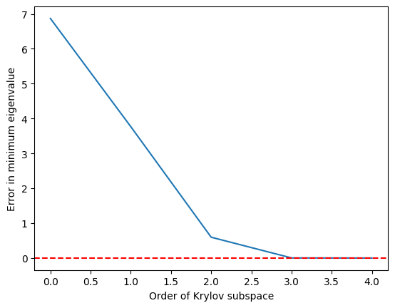
On constate que la valeur propre minimale est atteinte avec une bonne précision dès que le sous-espace de Krylov a grandi jusqu'à $\mathcal{K}^2,$ et est parfaite à partir de $\mathcal{K}^3.$

2.2 Mise à l'échelle temporelle selon la dimension de la matrice

Montrons que la méthode de Krylov peut être avantageuse par rapport aux solveurs de valeurs propres numériques exacts, de la façon suivante :

• Construire des matrices aléatoires (non creuses, pas l'application idéale pour KQD)
• Déterminer les valeurs propres par deux méthodes : directement avec NumPy et en utilisant un sous-espace de Krylov.
• Choisir un seuil de précision pour nos valeurs propres, avant d'accepter les estimations de Krylov.
• Comparer le temps d'exécution nécessaire pour résoudre le problème avec ces deux méthodes.

Mises en garde : Comme nous le discuterons en détail ci-dessous, la diagonalisation quantique de Krylov est mieux adaptée aux opérateurs dont les représentations matricielles sont creuses et/ou peuvent être écrites à l'aide d'un petit nombre de groupes d'opérateurs de Pauli commutants. Les matrices aléatoires que nous utilisons ici ne correspondent pas à ce profil. Elles ne servent qu'à sonder l'échelle à laquelle les méthodes de Krylov classiques peuvent être utiles. Deuxièmement, en utilisant la méthode de Krylov, nous calculerons les valeurs propres à l'aide de plusieurs sous-espaces de Krylov de tailles différentes. Nous rapporterons le temps nécessaire pour le sous-espace de Krylov de dimension minimale qui atteint la précision requise pour la valeur propre de l'état fondamental. Là encore, cela diffère un peu de la résolution d'un problème intraitable pour les solveurs exacts, puisque nous utilisons la solution exacte pour évaluer la dimension nécessaire.

Commençons par générer notre ensemble de matrices aléatoires.

import numpy as np

# Set the random seed
np.random.seed(42)

# how many random matrices will we make
num_matrix = 200

matrices = []
for m in range(1, num_matrix):
    matrices.append(np.random.rand(m, m))

Nous diagonalisons maintenant chaque matrice directement avec numpy. Nous calculons le temps nécessaire à la diagonalisation pour une comparaison ultérieure.

matrix_numpy_times = []
matrix_numpy_eigs = []
for mm in range(num_matrix - 1):
    t0 = time_mus()
    matrix_numpy_eigs.append(min(np.linalg.eig(matrices[mm]).eigenvalues))
    matrix_numpy_times.append(time_mus() - t0)

plt.plot(matrix_numpy_times)
plt.xlabel("Dimension of matrix")  # Add x-axis label
plt.ylabel("Time to diagonalize (microsec)")  # Add y-axis label
plt.show()

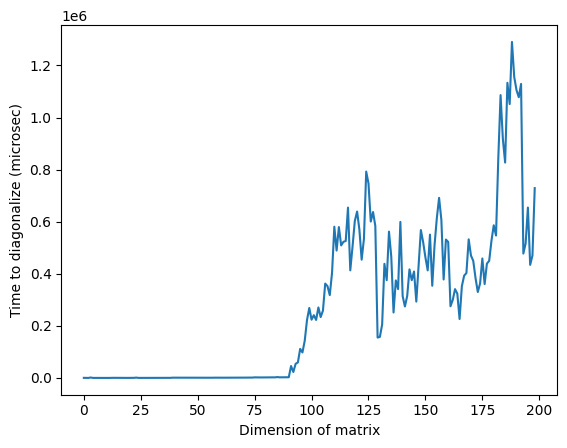
Remarque : dans l'image ci-dessus, le temps anormalement élevé autour d'une dimension de 125 peut être dû à la nature aléatoire des matrices ou à l'implémentation sur le processeur classique utilisé, mais il n'est pas reproductible. En relançant le code, on obtiendra un profil différent avec d'autres pics anormaux.

Maintenant, pour chaque matrice, nous construirons un sous-espace de Krylov et calculerons les valeurs propres par étapes. À chaque étape, nous vérifierons si la valeur propre la plus basse a été obtenue à l'intérieur de notre erreur absolue spécifiée. Le sous-espace qui nous donne en premier des valeurs propres dans notre marge d'erreur spécifiée est celui pour lequel nous enregistrerons les temps de calcul. L'exécution de cette cellule peut prendre plusieurs minutes, selon la vitesse du processeur. N'hésite pas à ignorer l'évaluation ou à réduire la dimension maximale des matrices diagonalisées. Consulter les résultats précalculés est suffisant.

# Choose the absolute error you can tolerate, and make a list for tracking the Krylov subspace size
# at which that error is achieved.
abserr = 0.05
accept_subspace_size = []

# Lists to store total time spent on the Krylov method, and the subset of that time spent on
# diagonalizing the projected matrix.
matrix_krylov_tot_times = []
matrix_krylov_dim = []

# Step through all our random matrices
for mm in range(0, num_matrix - 1):
    test_ks, test_Hs, test_eigs, test_k_tot_times = krylov_full_build(
        np.ones(len(matrices[mm])), matrices[mm]
    )
    # We have not yet found a Krylov subspace that produces our minimum eigenvalue to
    # within the required error.
    found = 0
    for j in range(0, len(matrices[mm]) - 1):
        # If we still haven't found the desired subspace...
        if found == 0:
            # ...but if this one satisfies the requirement, then record everything
            if (
                abs((min(test_eigs[j]) - matrix_numpy_eigs[mm]) / matrix_numpy_eigs[mm])
                < abserr
            ):
                accept_subspace_size.append(j)
                matrix_krylov_tot_times.append(test_k_tot_times[j])
                matrix_krylov_dim.append(mm)
                found = 1

Traçons les temps obtenus avec ces deux méthodes pour les comparer :

plt.plot(matrix_numpy_times, color="blue")
plt.plot(matrix_krylov_dim, matrix_krylov_tot_times, color="green")
plt.xlabel("Dimension of matrix")  # Add x-axis label
plt.ylabel("Time to diagonalize (microsec)")  # Add y-axis label
plt.show()

Ce sont les temps réels nécessaires, mais pour faciliter la discussion, lissons ces courbes en faisant la moyenne sur quelques points adjacents / dimensions de matrices. C'est ce qui est fait ci-dessous :

smooth_numpy_times = []
smooth_krylov_times = []

# Choose the number of adjacent points over which to average forward;
# the same will be used backward.
smooth_steps = 10

# We will do this smoothing for all points/matrix dimensions
for i in range(len(matrix_krylov_tot_times)):
    # Ensure we don't exceed the boundaries of our lists
    start = max(0, i - smooth_steps)
    end = min(len(matrix_krylov_tot_times) - 1, i + smooth_steps)

    # Dummy variables for accumulating an average over adjacent points. This is done for both Krylov
    # and the NumPy calculations.
    smooth_count = 0
    smooth_numpy_sum = 0
    smooth_krylov_sum = 0

    for j in range(start, end):
        smooth_numpy_sum = smooth_numpy_sum + matrix_numpy_times[j]
        smooth_krylov_sum = smooth_krylov_sum + matrix_krylov_tot_times[j]
        smooth_count = smooth_count + 1

    # Appending the averaged adjacent values to our new smooth lists
    smooth_numpy_times.append(smooth_numpy_sum / smooth_count)
    smooth_krylov_times.append(smooth_krylov_sum / smooth_count)

plt.plot(smooth_numpy_times, color="blue")
plt.plot(smooth_krylov_times, color="green")
plt.xlabel("Dimension of matrix")  # Add x-axis label
plt.ylabel("Time to diagonalize (smoothed, microsec)")  # Add y-axis label
plt.show()

On remarque que le temps nécessaire pour construire un sous-espace de Krylov dépasse initialement le temps requis pour la diagonalisation complète de numpy. Mais à mesure que la taille de la matrice augmente, la méthode de Krylov devient avantageuse. Cela est vrai même si l'on réduit notre erreur acceptable, mais l'avantage apparaît à une dimension de matrice plus grande. Il vaut la peine de décortiquer cela.

La complexité temporelle de la diagonalisation numérique est $O(n^3)$ (avec quelques variations selon les algorithmes). La complexité temporelle de la génération d'une base orthonormale de $n$ vecteurs est également $O(n^3)$. Donc l'avantage de la méthode de Krylov n'est pas lié à l'utilisation d'$\it{une quelconque}$ base orthonormale, mais à l'utilisation d'une base orthonormale particulière qui identifie efficacement les valeurs propres d'intérêt. Nous avons déjà vu cela dans l'esquisse de preuve de la première section de cette leçon, et c'est essentiel pour les garanties de convergence des méthodes de Krylov.

Résumons les progrès accomplis jusqu'ici :

• Pour les très grandes matrices, la méthode du sous-espace de Krylov peut fournir des valeurs propres approximatives dans les tolérances requises plus rapidement que les algorithmes de diagonalisation traditionnels.
• Pour de telles très grandes matrices, la génération d'un sous-espace de Krylov est la partie la plus chronophage de la méthode du sous-espace de Krylov.
• Ainsi, une méthode efficace pour générer un sous-espace de Krylov serait extrêmement précieuse.

C'est là qu'intervient enfin l'ordinateur quantique.

Vérifie ta compréhension

Consulte le graphique lissé des temps de diagonalisation par rapport à la dimension de la matrice ci-dessus.

(a) À quelle dimension de matrice approximative la méthode de Krylov est-elle devenue plus rapide, selon ce graphique ?

(b) Quels aspects du calcul pourraient modifier cette dimension à laquelle la méthode de Krylov devient plus rapide ?

Answer

(a) Les réponses peuvent varier si tu relances le calcul, mais la méthode de Krylov devient plus rapide à une dimension d'environ 80-85.

(b) Il existe de nombreuses réponses possibles. Parmi les facteurs importants, on trouve la précision requise et la creusité des matrices à diagonaliser.

3. Krylov via l'évolution temporelle

Tout ce que nous avons décrit jusqu'ici peut être réalisé classiquement. Alors comment et quand utiliserait-on un ordinateur quantique ? Pour de très grandes matrices, la méthode de Krylov peut nécessiter de longs temps de calcul et de grandes quantités de mémoire. Le temps requis pour l'opération matricielle de $H$ sur $|v\rangle$ évolue comme $O(N^2)$ dans le pire des cas. Même la multiplication de matrices creuses par un vecteur (le cas typique pour les solveurs de type Krylov classiques) a une complexité temporelle qui évolue comme $O(N)$. Cette opération est répétée pour chaque vecteur que l'on souhaite intégrer dans notre sous-espace. La dimension du sous-espace $r$ n'est généralement pas une fraction significative de $N$, et évolue souvent comme $\log(N)$. Ainsi, la génération de tous les vecteurs évolue comme $O(N^2 \log(N))$ dans le pire des cas. Bien qu'il existe d'autres étapes, comme l'orthogonalisation, c'est l'évolution dominante à garder à l'esprit.

L'informatique quantique nous permet de modifier les attributs du problème qui déterminent l'évolution du temps et des ressources nécessaires. Au lieu d'une dépendance à la taille de la matrice $N$ dans tous les cas, on verra apparaître des éléments comme le nombre de shots et le nombre de termes de Pauli non commutatifs composant le Hamiltonien. Voyons comment cela fonctionne.

3.1 L'évolution temporelle

Rappelle-toi que l'opérateur qui fait évoluer temporellement un état quantique est $e^{-iHt/\hbar}$ (et il est très courant, surtout en informatique quantique, d'omettre le $\hbar$ de la notation). Une façon de comprendre et même de réaliser une telle fonction exponentielle d'un opérateur est d'examiner son développement en série de Taylor. Note que cette opération appliquée à un vecteur initial $|v\rangle$ produit une somme de termes avec des puissances croissantes de $H$ appliquées à l'état initial. On dirait que l'on peut simplement construire notre sous-espace de Krylov en faisant évoluer temporellement notre état initial de référence !

$$\begin{aligned} e^{-iHt/\hbar}→e^{-iHt}&≈1-iHt-\frac{(H^2 t^2)}{2}+⋯\\ e^{-iHt} |v\rangle &≈ |v\rangle-iHt|v\rangle-\frac{(H^2 t^2)}{2}|v\rangle+⋯ \end{aligned}$$

La difficulté réside dans la réalisation de l'évolution temporelle sur un vrai ordinateur quantique. Beaucoup des termes du Hamiltonien ne commutent pas entre eux. Ainsi, si certains opérateurs exponentiels simples comme $e^{-iZ}$ correspondent à des circuits simples, les Hamiltoniens généraux, eux, n'en ont pas. Et puisqu'ils contiennent des termes non commutatifs, on ne peut pas simplement décomposer l'exponentielle en un produit de termes simples, comme on le ferait avec des nombres.

$$e^{-iHt}=e^{-i(H_1+H_2+⋯+H_n)t}\neq e^{-iH_1 t} e^{-iH_2 t}... e^{-iH_n t}$$

Ce n'est donc pas trivial, mais c'est un processus bien étudié en informatique quantique. On réalise l'évolution temporelle sur des ordinateurs quantiques à l'aide d'un processus appelé trotterisation, qui est en soi un sujet riche[10]. Mais à très haut niveau, en décomposant l'évolution temporelle en très petits pas, disons $m$ pas de taille $dt$, on limite les effets de la non-commutativité des termes.

$$e^{-iHt}=e^{-i(H_1+H_2+⋯+H_n )t} = (e^{-i(H_1+H_2+⋯+H_n )t/m} )^m ≈(e^{-iH_1 dt} e^{-iH_2 dt} …e^{-iH_n dt} )^m$$

où $dt = t/m$.

Appelons sous-espace de Krylov de puissance un sous-espace de Krylov d'ordre r que nous avons généré dans le contexte classique en utilisant directement les puissances de H.

$$\mathcal{K}_P^r (H,|v\rangle)=\text{span}\{|v\rangle,H|v\rangle,H^2 |v\rangle… H^{r-1} |v\rangle\}$$

On génère maintenant un espace similaire en utilisant l'opérateur d'évolution temporelle unitaire $U \equiv e^{-iHt}$ ; on appellera cet espace le "sous-espace de Krylov unitaire" $\mathcal{K}_U^r$. Le sous-espace de Krylov de puissance $\mathcal{K}_P^r$ que l'on utilise classiquement ne peut pas être généré directement sur un ordinateur quantique, car $H$ n'est pas un opérateur unitaire. Il a été démontré que l'utilisation du sous-espace de Krylov unitaire offre des garanties de convergence similaires à celles du sous-espace de Krylov de puissance, à savoir que l'erreur sur l'état fondamental converge efficacement tant que l'état initial $|v\rangle$ a un recouvrement avec le vrai état fondamental qui ne s'annule pas exponentiellement, et tant qu'il existe un écart suffisant entre les valeurs propres. Voir la Réf [1] pour une discussion plus précise de la convergence.

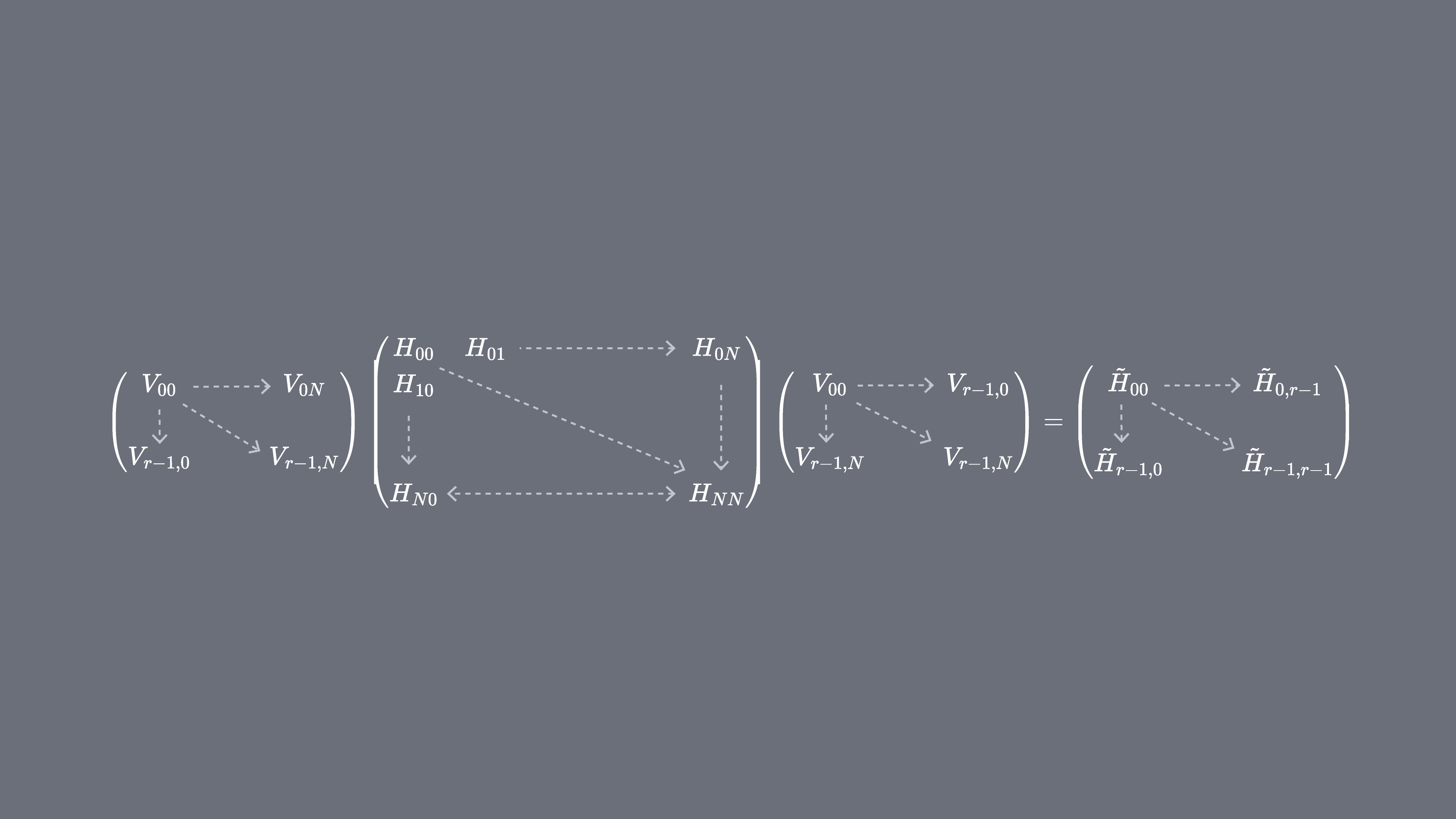
Ici, les puissances de $U$ correspondent à différents pas de temps (la $k^\text{ième}$ puissance de $U$ correspond à un avancement de $k \times dt$). On peut nommer l'élément du sous-espace dont l'évolution temporelle totale est $k dt$ par $|\psi_k\rangle$.

$$\begin{aligned} U&=e^{-iHdt}\\ U^k&=e^{-iH(kdt)}\\ \mathcal{K}_U^r&=\text{span}\{|\psi\rangle,U|\psi\rangle,U^2 |\psi\rangle… U^{r-1} |\psi\rangle\} \end{aligned}$$

On peut projeter notre Hamiltonien H sur le sous-espace de Krylov unitaire, $\mathcal{K}_U^r$. Autrement dit, on calcule chaque élément de matrice de $H$ dans la base $\mathcal{K}_U^r$. On désignera cette matrice projetée par $\tilde{H}$.

3.2 Comment l'implémenter sur un ordinateur quantique

Les éléments de matrice de $\tilde{H}$ sont donnés par les valeurs d'espérance $\langle \psi_m |H| \psi_n\rangle$, qui peuvent être estimées à l'aide de l'ordinateur quantique. Garde à l'esprit que $H$ peut s'écrire comme une somme d'opérateurs de Pauli sur différents qubits, et que tous les opérateurs de Pauli ne peuvent pas être mesurés simultanément. On peut regrouper les termes de Pauli en groupes de termes commutatifs et mesurer tous ceux-là en même temps. Mais il peut être nécessaire de former de nombreux groupes de ce type pour couvrir tous les termes. Le nombre de groupes commutatifs distincts en lesquels les termes peuvent être partitionnés, $N_\text{GCP}$, devient donc important.

$$H=\sum_{\alpha=1}^{N_\text{GCP}} c_\alpha P_\alpha$$

Ici, $P_\alpha$ est une chaîne de Pauli de la forme $P_\alpha \sim IZIXII...YZXIX$ ou un ensemble de telles chaînes de Pauli qui commutent entre elles. Étant donné que l'on peut écrire $H$ comme une telle somme d'opérateurs mesurables, les expressions suivantes pour les éléments de matrice de $\tilde{H}$ peuvent être réalisées à l'aide du primitif Estimator de Qiskit Runtime.

$$\begin{aligned} \tilde{H}_{mn}&=\langle \psi_m |H| \psi_n\rangle\\ &=\langle \psi e^{iHt_m} |H| \psi e^{-iHt_n}\rangle\\ &=\langle \psi e^{iHmdt} |H|\psi e^{-iHndt}\rangle \end{aligned}$$

Où $\vert \psi_n \rangle = e^{-i H t_n} \vert \psi \rangle$ sont les vecteurs du sous-espace de Krylov unitaire et $t_n = n dt$ sont les multiples du pas de temps $dt$ choisi. Sur un ordinateur quantique, le calcul de chaque élément de matrice peut être réalisé avec n'importe quel algorithme permettant d'obtenir le recouvrement entre des états quantiques. Dans cette leçon, on se concentrera sur le test de Hadamard. Étant donné que $\mathcal{K}_U$ a une dimension $r$, le Hamiltonien projeté dans le sous-espace aura des dimensions $r \times r$. Avec $r$ suffisamment petit (généralement $r<<100$ suffit pour obtenir la convergence des estimations des valeurs propres), on peut alors facilement diagonaliser classiquement le Hamiltonien projeté $\tilde{H}$. Cependant, on ne peut pas diagonaliser directement $\tilde{H}$ en raison de la non-orthogonalité des vecteurs du sous-espace de Krylov. Il faut mesurer leurs recouvrements et construire une matrice $\tilde{S}$

$$\tilde{S}_{mn} = \langle \psi_m \vert \psi_n \rangle$$

Cela nous permet de résoudre le problème aux valeurs propres dans un espace non orthogonal (aussi appelé problème aux valeurs propres généralisé)

$$\tilde{H} \ \vec{c} = E \ \tilde{S} \ \vec{c}$$

On peut ensuite obtenir des estimations des valeurs propres et des états propres de $H$ en examinant les solutions de ce problème aux valeurs propres généralisé. Par exemple, l'estimation de l'énergie de l'état fondamental s'obtient en prenant la plus petite valeur propre $E$ et l'état fondamental à partir du vecteur propre correspondant $\vec{c}$. Les coefficients dans $\vec{c}$ déterminent la contribution des différents vecteurs qui forment l'espace $\mathcal{K}_U$.

Problème aux valeurs propres généralisé

Pourquoi ne peut-on pas simplement diagonaliser $\tilde{H}$ ? Puisque $\tilde{S}$ contient l'information sur la géométrie de la base de Krylov (qui est non orthogonale sauf dans des cas très particuliers), $\tilde{H}$ seul ne décrit pas une projection du Hamiltonien complet, donc ses valeurs propres n'ont aucune relation particulière avec celles du Hamiltonien complet — elles pourraient être des valeurs quelconques. La résolution du problème aux valeurs propres généralisé est nécessaire pour obtenir les valeurs propres et vecteurs propres approximatifs correspondant à la projection du Hamiltonien complet dans le sous-espace de Krylov.

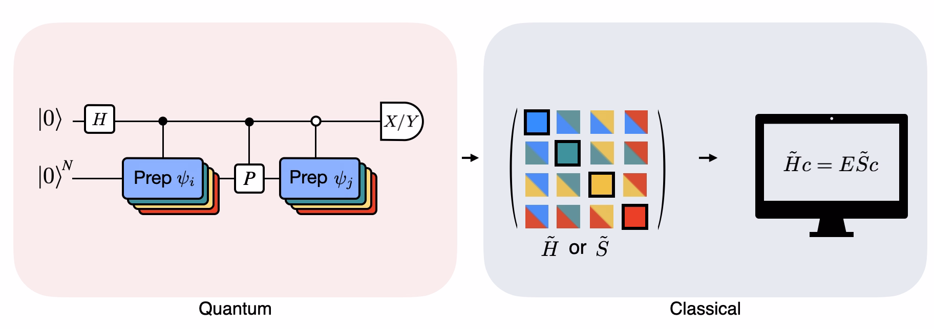
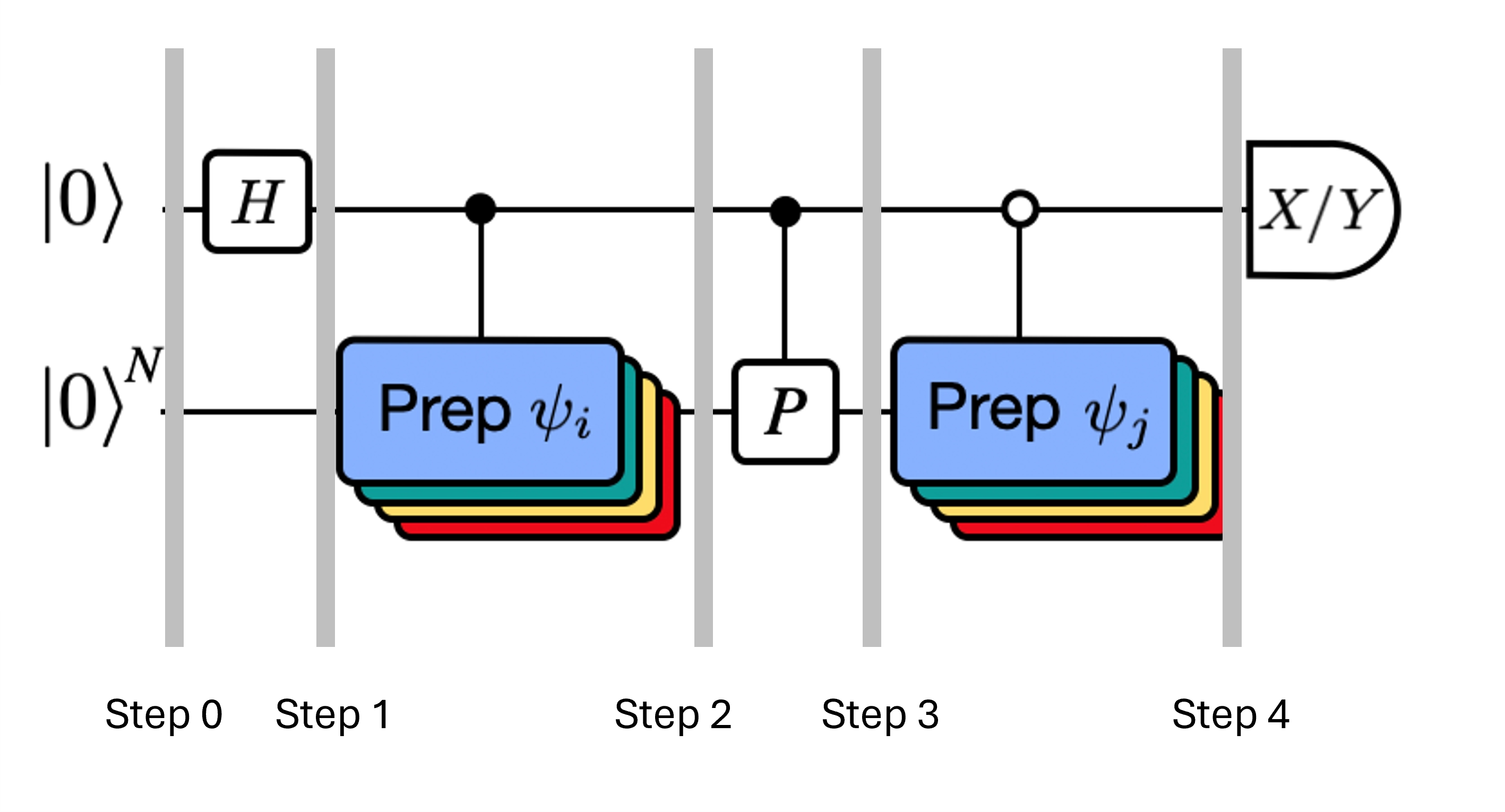
La figure montre une représentation sous forme de circuit du test de Hadamard modifié, une méthode utilisée pour calculer le recouvrement entre différents états quantiques. Pour chaque élément de matrice $\tilde{H}_{i,j}$, un test de Hadamard entre les états $\vert \psi_i \rangle$, $\vert \psi_j \rangle$ est effectué. Ceci est mis en évidence dans la figure par le code couleur des éléments de matrice et les opérations $\text{Prep} \; \psi_i$, $\text{Prep} \; \psi_j$ correspondantes. Ainsi, un ensemble de tests de Hadamard pour toutes les combinaisons possibles de vecteurs du sous-espace de Krylov est nécessaire pour calculer tous les éléments de matrice du Hamiltonien projeté $\tilde{H}$. Le fil supérieur dans le circuit du test de Hadamard est un qubit ancilla qui est mesuré soit dans la base X, soit dans la base Y ; sa valeur d'espérance détermine la valeur du recouvrement entre les états. Le fil inférieur représente tous les qubits du Hamiltonien du système. L'opération $\text{Prep} \; \psi_i$ prépare le qubit du système dans l'état $\vert \psi_i \rangle$ contrôlé par l'état du qubit ancilla (de même pour $\text{Prep} \; \psi_j$) et l'opération $P$ représente la décomposition de Pauli du Hamiltonien du système $H = \sum_i P_i$. L'implémentation de ceci sur un ordinateur quantique est présentée plus en détail ci-dessous.

4. Diagonalisation quantique de Krylov sur un ordinateur quantique

On va maintenant implémenter la diagonalisation quantique de Krylov sur un vrai ordinateur quantique. Commençons par importer quelques packages utiles.

import numpy as np
import scipy as sp
import matplotlib.pylab as plt
from typing import Union, List
import warnings

from qiskit.quantum_info import SparsePauliOp, Pauli
from qiskit.circuit import Parameter
from qiskit import QuantumCircuit, QuantumRegister
from qiskit.circuit.library import PauliEvolutionGate
from qiskit.synthesis import LieTrotter

# from qiskit.providers.fake_provider import Fake20QV1
from qiskit_ibm_runtime import QiskitRuntimeService, EstimatorV2 as Estimator, Batch

import itertools as it

warnings.filterwarnings("ignore")

On définit la fonction ci-dessous pour résoudre le problème aux valeurs propres généralisé que l'on vient d'expliquer.

def solve_regularized_gen_eig(
    h: np.ndarray,
    s: np.ndarray,
    threshold: float,
    k: int = 1,
    return_dimn: bool = False,
) -> Union[float, List[float]]:
    """
    Method for solving the generalized eigenvalue problem with regularization

    Args:
        h (numpy.ndarray):
            The effective representation of the matrix in our Krylov subspace
        s (numpy.ndarray):
            The matrix of overlaps between vectors of our Krylov subspace
        threshold (float):
            Cut-off value for the eigenvalue of s
        k (int):
            Number of eigenvalues to return
        return_dimn (bool):
            Whether to return the size of the regularized subspace

    Returns:
        lowest k-eigenvalue(s) that are the solution of the regularized generalized eigenvalue problem

    """
    s_vals, s_vecs = sp.linalg.eigh(s)
    s_vecs = s_vecs.T
    good_vecs = np.array([vec for val, vec in zip(s_vals, s_vecs) if val > threshold])
    h_reg = good_vecs.conj() @ h @ good_vecs.T
    s_reg = good_vecs.conj() @ s @ good_vecs.T
    if k == 1:
        if return_dimn:
            return sp.linalg.eigh(h_reg, s_reg)[0][0], len(good_vecs)
        else:
            return sp.linalg.eigh(h_reg, s_reg)[0][0]
    else:
        if return_dimn:
            return sp.linalg.eigh(h_reg, s_reg)[0][:k], len(good_vecs)
        else:
            return sp.linalg.eigh(h_reg, s_reg)[0][:k]

Au moins lors d'un premier benchmarking, il est utile de connaître une solution classique exacte pour vérifier le comportement de convergence. La fonction ci-dessous calcule l'énergie de l'état fondamental d'un Hamiltonien, en prenant le Hamiltonien et le nombre de qubits comme arguments.

def single_particle_gs(H_op, n_qubits):
    """
    Find the ground state of the single particle(excitation) sector
    """
    H_x = []
    for p, coeff in H_op.to_list():
        H_x.append(set([i for i, v in enumerate(Pauli(p).x) if v]))

    H_z = []
    for p, coeff in H_op.to_list():
        H_z.append(set([i for i, v in enumerate(Pauli(p).z) if v]))

    H_c = H_op.coeffs

    print("n_sys_qubits", n_qubits)

    n_exc = 1
    sub_dimn = int(sp.special.comb(n_qubits + 1, n_exc))
    print("n_exc", n_exc, ", subspace dimension", sub_dimn)

    few_particle_H = np.zeros((sub_dimn, sub_dimn), dtype=complex)

    sparse_vecs = [
        set(vec) for vec in it.combinations(range(n_qubits + 1), r=n_exc)
    ]  # list all of the possible sets of n_exc indices of 1s in n_exc-particle states

    m = 0
    for i, i_set in enumerate(sparse_vecs):
        for j, j_set in enumerate(sparse_vecs):
            m += 1

            if len(i_set.symmetric_difference(j_set)) <= 2:
                for p_x, p_z, coeff in zip(H_x, H_z, H_c):
                    if i_set.symmetric_difference(j_set) == p_x:
                        sgn = ((-1j) ** len(p_x.intersection(p_z))) * (
                            (-1) ** len(i_set.intersection(p_z))
                        )
                    else:
                        sgn = 0

                    few_particle_H[i, j] += sgn * coeff

    gs_en = min(np.linalg.eigvalsh(few_particle_H))
    print("single particle ground state energy: ", gs_en)
    return gs_en

4.1 Étape 1 : Mapper le problème sur des circuits quantiques et des opérateurs

On va maintenant définir un Hamiltonien. Cela est distinct de la fonction ci-dessus, qui prend un Hamiltonien comme argument et ne retourne que l'état fondamental, et ce de manière classique. Ce Hamiltonien que l'on définit ici détermine les niveaux d'énergie de tous les états propres d'énergie, et ce Hamiltonien peut être construit à l'aide d'opérateurs de Pauli et implémenté sur un ordinateur quantique.

On choisit un Hamiltonien correspondant à une chaîne de spins pouvant avoir n'importe quelle orientation dans l'espace, appelée "chaîne de Heisenberg". On suppose que le $i^\text{ième}$ spin peut être influencé par ses plus proches voisins (les $(i-1)^\text{ième}$ et $(i+1)^\text{ième}$ spins) mais pas par des voisins plus éloignés. On autorise également la possibilité que l'interaction entre les spins soit différente selon les axes le long desquels ils pointent. Cette asymétrie survient parfois, par exemple, en raison de la structure du réseau cristallin dans lequel les spins sont intégrés.

# Define problem Hamiltonian.
n_qubits = 10
# coupling strength for XX, YY, and ZZ interactions
JX = 1
JY = 3
JZ = 2

# Define the Hamiltonian:
H_int = [["I"] * n_qubits for _ in range(3 * (n_qubits - 1))]
for i in range(n_qubits - 1):
    H_int[i][i] = "Z"
    H_int[i][i + 1] = "Z"
for i in range(n_qubits - 1):
    H_int[n_qubits - 1 + i][i] = "X"
    H_int[n_qubits - 1 + i][i + 1] = "X"
for i in range(n_qubits - 1):
    H_int[2 * (n_qubits - 1) + i][i] = "Y"
    H_int[2 * (n_qubits - 1) + i][i + 1] = "Y"
H_int = ["".join(term) for term in H_int]
H_tot = [
    (term, JZ)
    if term.count("Z") == 2
    else (term, JY)
    if term.count("Y") == 2
    else (term, JX)
    for term in H_int
]

# Get operator
H_op = SparsePauliOp.from_list(H_tot)
print(H_tot)

[('ZZIIIIIIII', 2), ('IZZIIIIIII', 2), ('IIZZIIIIII', 2), ('IIIZZIIIII', 2), ('IIIIZZIIII', 2), ('IIIIIZZIII', 2), ('IIIIIIZZII', 2), ('IIIIIIIZZI', 2), ('IIIIIIIIZZ', 2), ('XXIIIIIIII', 1), ('IXXIIIIIII', 1), ('IIXXIIIIII', 1), ('IIIXXIIIII', 1), ('IIIIXXIIII', 1), ('IIIIIXXIII', 1), ('IIIIIIXXII', 1), ('IIIIIIIXXI', 1), ('IIIIIIIIXX', 1), ('YYIIIIIIII', 3), ('IYYIIIIIII', 3), ('IIYYIIIIII', 3), ('IIIYYIIIII', 3), ('IIIIYYIIII', 3), ('IIIIIYYIII', 3), ('IIIIIIYYII', 3), ('IIIIIIIYYI', 3), ('IIIIIIIIYY', 3)]

Le code ci-dessous restreint le Hamiltonien aux états à une seule particule, et utilise la norme spectrale pour définir une bonne taille pour notre pas de temps $dt$. On choisit heuristiquement une valeur pour le pas de temps dt (basée sur des bornes supérieures de la norme du Hamiltonien). La Réf [9] a montré qu'un pas de temps suffisamment petit est $\pi/\vert \vert H \vert \vert$, et qu'il est préférable, jusqu'à un certain point, de sous-estimer cette valeur plutôt que de la surestimer, car une surestimation peut permettre aux contributions des états de haute énergie de corrompre même l'état optimal dans le sous-espace de Krylov. D'un autre côté, choisir $dt$ trop petit conduit à un mauvais conditionnement du sous-espace de Krylov, car les vecteurs de la base de Krylov diffèrent moins d'un pas de temps à l'autre.

# Get Hamiltonian restricted to single-particle states
single_particle_H = np.zeros((n_qubits, n_qubits))
for i in range(n_qubits):
    for j in range(i + 1):
        for p, coeff in H_op.to_list():
            p_x = Pauli(p).x
            p_z = Pauli(p).z
            if all(p_x[k] == ((i == k) + (j == k)) % 2 for k in range(n_qubits)):
                sgn = ((-1j) ** sum(p_z[k] and p_x[k] for k in range(n_qubits))) * (
                    (-1) ** p_z[i]
                )
            else:
                sgn = 0
            single_particle_H[i, j] += sgn * coeff
for i in range(n_qubits):
    for j in range(i + 1, n_qubits):
        single_particle_H[i, j] = np.conj(single_particle_H[j, i])

# Set dt according to spectral norm
dt = np.pi / np.linalg.norm(single_particle_H, ord=2)
dt

np.float64(0.17453292519943295)

On précise le nombre de pas de Trotter à utiliser dans l'évolution temporelle. On précise également une dimension maximale de Krylov de 4. Cette dimension de Krylov n'est pas suffisamment grande pour des applications réalistes. Mais elle est suffisante pour cet exemple. De plus, on vérifiera la convergence à des dimensions encore plus petites. On explorera dans des leçons ultérieures des méthodes qui nous permettront de mettre à l'échelle et de projeter nos Hamiltoniens sur des sous-espaces plus grands.

# Set parameters for quantum Krylov algorithm
krylov_dim = 4  # size of krylov subspace
num_trotter_steps = 4
dt_circ = dt / num_trotter_steps

Préparation de l'état

Choisis un état de référence $\vert \psi \rangle$ ayant un certain recouvrement avec l'état fondamental. Pour ce Hamiltonien, on utilise un état avec une excitation dans le qubit central $\vert 00..010...00 \rangle$ comme état de référence.

qc_state_prep = QuantumCircuit(n_qubits)
qc_state_prep.x(int(n_qubits / 2) + 1)
qc_state_prep.draw("mpl", scale=0.5)

Évolution temporelle

On peut réaliser l'opérateur d'évolution temporelle généré par un Hamiltonien donné : $U=e^{-iHt}$ via l'approximation de Lie-Trotter. Pour simplifier, on utilise la PauliEvolutionGate intégrée dans le circuit d'évolution temporelle. La syntaxe générale pour cela est la suivante.

t = Parameter("t")

## Create the time-evo op circuit
evol_gate = PauliEvolutionGate(
    H_op, time=t, synthesis=LieTrotter(reps=num_trotter_steps)
)

qr = QuantumRegister(n_qubits)
qc_evol = QuantumCircuit(qr)
qc_evol.append(evol_gate, qargs=qr)

<qiskit.circuit.instructionset.InstructionSet at 0x7ccaa4664250>

Nous utiliserons une version de ce circuit ci-dessous dans le test de Hadamard, en avançant d'un pas de temps $dt$.

Test de Hadamard

Rappelle-toi que nous souhaitons calculer les éléments de matrice de $\tilde{H}$ et de la matrice de Gram $\tilde{S}$ à l'aide du test de Hadamard. Voyons comment cela fonctionne dans ce contexte, en nous concentrant d'abord sur la construction de $\tilde{H}.$ Le processus global est représenté graphiquement ci-dessous. Les couches de blocs de préparation d'état colorés $\text{Prep}|\psi_i\rangle$ servent de rappel que ce processus est effectué pour toutes les combinaisons de $|\psi_i\rangle$ et $|\psi_j\rangle$ dans notre sous-espace.

Les états du système aux étapes indiquées sont :

$$\begin{aligned} \text{Step 0:}\qquad|\Psi\rangle & = |0\rangle|0\rangle^N \\ \text{Step 1:}\qquad|\Psi\rangle & = \frac{1}{\sqrt{2}}\Big(|0\rangle + |1\rangle \Big)|0\rangle^N \\ \text{Step 2:}\qquad|\Psi\rangle & = \frac{1}{\sqrt{2}}\Big(|0\rangle|0\rangle^N+|1\rangle |\psi_i\rangle\Big)\\ \text{Step 3:}\qquad|\Psi\rangle & = \frac{1}{\sqrt{2}}\Big(|0\rangle |0\rangle^N+|1\rangle P |\psi_i\rangle\Big) \\ \text{Step 4:}\qquad|\Psi\rangle & = \frac{1}{\sqrt{2}}\Big(|0\rangle |\psi_j\rangle+|1\rangle P|\psi_i\rangle\Big) \end{aligned}$$

Ici $P$ est un terme de Pauli dans la décomposition du hamiltonien (note qu'il ne peut pas s'agir d'une combinaison linéaire de plusieurs termes de Pauli qui commutent, car ce ne serait pas unitaire — le regroupement est possible en utilisant une construction différente que nous montrerons plus tard) $\text{Prep} \; \psi_i$, $\text{Prep} \; \psi_j$ sont des opérations contrôlées qui préparent les vecteurs $|\psi_i\rangle$, $|\psi_j\rangle$ de l'espace de Krylov unitaire, avec $|\psi_k\rangle = e^{-i H k dt } \vert \psi \rangle = e^{-i H k dt } U_{\psi} \vert 0 \rangle^N$. Appliquer des mesures de $X$ et $Y$ à ce circuit calcule respectivement les parties réelle et imaginaire des éléments de matrice dont nous avons besoin.

En partant de l'étape 4 ci-dessus, applique la porte Hadamard $H$ au qubit zéro.

$$\begin{equation*} |\Psi\rangle \longrightarrow\quad\frac{1}{2}|0\rangle\Big( |\psi_j\rangle + P|\psi_i\rangle\Big) + \frac{1}{2}|1\rangle\Big(|\psi_j\rangle - P|\psi_i\rangle\Big) \end{equation*}$$

Mesure ensuite soit $X$ soit $Y$.

$$\begin{equation*} \begin{split} \Rightarrow\quad\langle X\rangle &= \frac{1}{4}\Bigg(\Big\|| \psi_j\rangle + P|\psi_i\rangle \Big\|^2-\Big\||\psi_j\rangle - P|\psi_i\rangle\Big\|^2\Bigg) \\ &= \text{Re}\Big[\langle\psi_j| P|\psi_i\rangle\Big]. \end{split} \end{equation*}$$

D'après l'identité $|a + b\|^2 = \langle a + b | a + b \rangle = \|a\|^2 + \|b\|^2 + 2\text{Re}\langle a | b \rangle$. De même, mesurer $Y$ donne

$$\begin{equation*} \langle Y\rangle = \text{Im}\Big[\langle\psi_j| P|\psi_i\rangle\Big]. \end{equation*}$$

En ajoutant ces étapes à l'évolution temporelle mise en place précédemment, on écrit ce qui suit.

## Create the time-evo op circuit
evol_gate = PauliEvolutionGate(
    H_op, time=dt, synthesis=LieTrotter(reps=num_trotter_steps)
)

## Create the time-evo op dagger circuit
evol_gate_d = PauliEvolutionGate(
    H_op, time=dt, synthesis=LieTrotter(reps=num_trotter_steps)
)
evol_gate_d = evol_gate_d.inverse()

# Put pieces together
qc_reg = QuantumRegister(n_qubits)
qc_temp = QuantumCircuit(qc_reg)
qc_temp.compose(qc_state_prep, inplace=True)
for _ in range(num_trotter_steps):
    qc_temp.append(evol_gate, qargs=qc_reg)
for _ in range(num_trotter_steps):
    qc_temp.append(evol_gate_d, qargs=qc_reg)
qc_temp.compose(qc_state_prep.inverse(), inplace=True)

# Create controlled version of the circuit
controlled_U = qc_temp.to_gate().control(1)

# Create hadamard test circuit for real part
qr = QuantumRegister(n_qubits + 1)
qc_real = QuantumCircuit(qr)
qc_real.h(0)
qc_real.append(controlled_U, list(range(n_qubits + 1)))
qc_real.h(0)

print("Circuit for calculating the real part of the overlap in S via Hadamard test")
qc_real.draw("mpl", fold=-1, scale=0.5)

Circuit for calculating the real part of the overlap in S via Hadamard test

Nous avons déjà averti de la profondeur impliquée dans les circuits de Trotter. Effectuer le test de Hadamard dans ces conditions peut produire un circuit encore plus profond, surtout une fois décomposé en portes natives. Cette profondeur augmentera encore davantage si l'on tient compte de la topologie du dispositif. Avant d'utiliser du temps de calcul sur l'ordinateur quantique, il est donc judicieux de vérifier la profondeur à 2 qubits de notre circuit.

print(
    "Number of layers of 2Q operations",
    qc_real.decompose(reps=2).depth(lambda x: x[0].num_qubits == 2),
)

Number of layers of 2Q operations 14401

Un circuit d'une telle profondeur ne peut pas produire de résultats exploitables sur les ordinateurs quantiques modernes. Si nous voulons construire $\tilde{H}$ et $\tilde{S},$ il nous faut une meilleure approche. C'est la raison pour laquelle le test de Hadamard efficace est introduit ci-dessous.

4. 2 Étape 2. Optimiser les circuits et les opérateurs pour le matériel cible

Test de Hadamard efficace

Nous pouvons optimiser les circuits profonds du test de Hadamard obtenus en introduisant quelques approximations et en nous appuyant sur certaines hypothèses concernant le hamiltonien du modèle. Par exemple, considère le circuit suivant pour le test de Hadamard :

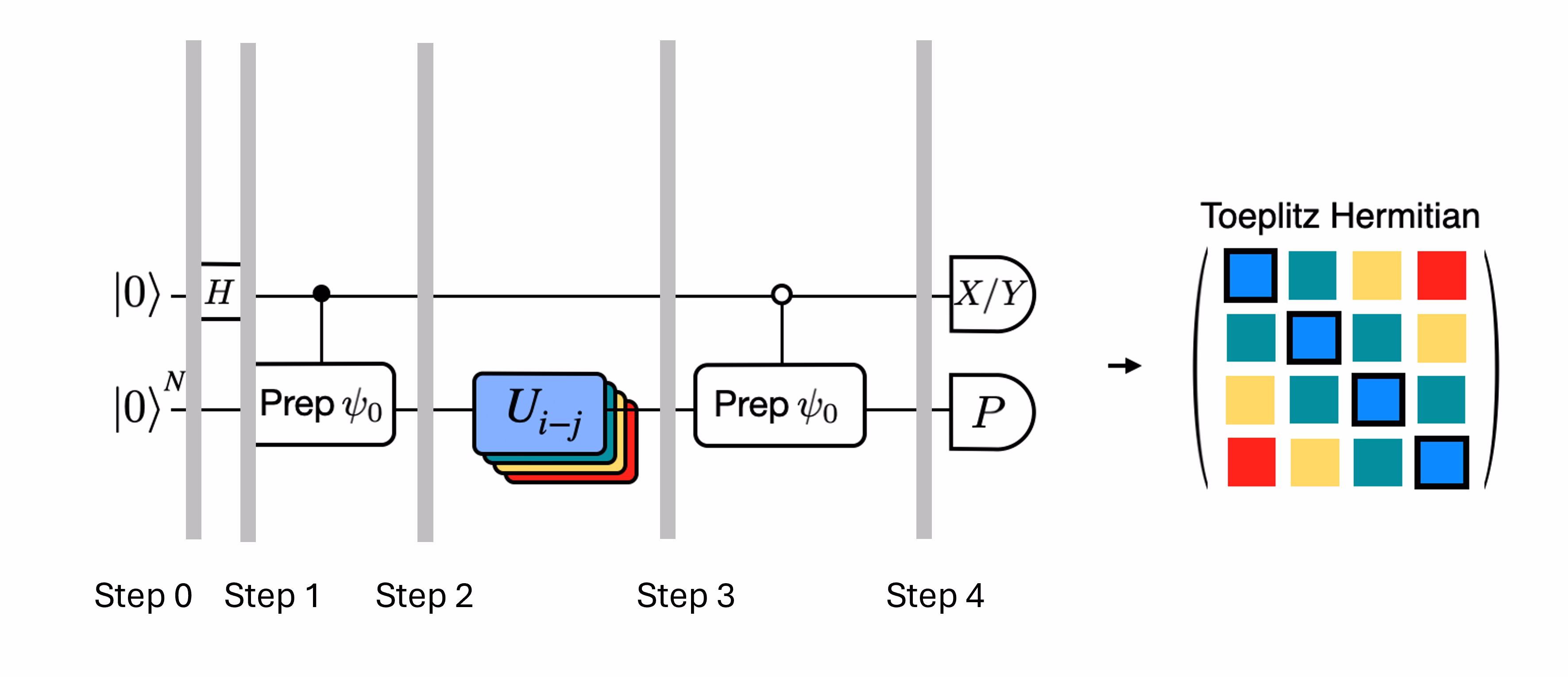
Supposons que nous puissions calculer classiquement $E_0$, la valeur propre de $|0\rangle^N$ sous le hamiltonien $H$. Cette condition est satisfaite lorsque le hamiltonien préserve la symétrie U(1). Même si cela peut sembler une hypothèse forte, il existe de nombreux cas où l'on peut supposer sans risque qu'il existe un état vide (qui correspond ici à l'état $|0\rangle^N$) non affecté par l'action du hamiltonien. C'est vrai, par exemple, pour les hamiltoniens de chimie décrivant une molécule stable (où le nombre d'électrons est conservé). Étant donné que la porte $\text{Prep} \; \psi_0$ prépare l'état de référence souhaité $\ket{\psi_0} = \text{Prep} \; \psi_0 \ket{0} = e^{-i H 0 dt} U_{\psi_0} \ket{0}$, par exemple pour préparer l'état HF en chimie, $\text{Prep} \; \psi_0$ serait un produit de NOT sur un seul qubit, de sorte que $\text{Prep} \; \psi_0$ contrôlé est simplement un produit de CNOT. Le circuit ci-dessus implémente alors l'état suivant avant la mesure :

$$\begin{aligned} \text{Step 0:}\qquad|\Psi\rangle & = \ket{0} \ket{0}^{N}\\ \text{Step 1:}\qquad|\Psi\rangle & = \frac{1}{\sqrt{2}}\left(\ket{0}\ket{0}^N+ \ket{1} \ket{0}^N\right)\\ \text{Step 2:}\qquad|\Psi\rangle & = \frac{1}{\sqrt{2}}\left(|0\rangle|0\rangle^N+|1\rangle|\psi_0\rangle\right)\\ \text{Step 3:}\qquad|\Psi\rangle & = \frac{1}{\sqrt{2}}\left(e^{i\phi}\ket{0}\ket{0}^N+\ket{1} U\ket{\psi_0}\right)\\ \text{Step 4:}\qquad|\Psi\rangle & = \frac{1}{\sqrt{2}}\left(e^{i\phi}\ket{0} \ket{\psi_0}+\ket{1} U\ket{\psi_0}\right)\\ & = \frac{1}{2}\left(\ket{+}\left(e^{i\phi}\ket{\psi_0}+U\ket{\psi_0}\right)+\ket{-}\left(e^{i\phi}\ket{\psi_0}-U\ket{\psi_0}\right)\right)\\ & = \frac{1}{2}\left(\ket{+i}\left(e^{i\phi}\ket{\psi_0}-iU\ket{\psi_0}\right)+\ket{-i}\left(e^{i\phi}\ket{\psi_0}+iU\ket{\psi_0}\right)\right) \end{aligned}$$

où nous avons utilisé le déphasage classiquement simulable $U\ket{0}^N = e^{i\phi}\ket{0}^N$ de l'étape 2 à 3. Les valeurs d'espérance sont donc

$$\begin{aligned} \langle X\otimes P\rangle&=\frac{1}{4} \Big( \left(e^{-i\phi}\bra{\psi_0}+\bra{\psi_0}U^\dagger\right)P\left(e^{i\phi}\ket{\psi_0}+U\ket{\psi_0}\right) \\ &\qquad-\left(e^{-i\phi}\bra{\psi_0}-\bra{\psi_0}U^\dagger\right)P\left(e^{i\phi}\ket{\psi_0}-U\ket{\psi_0}\right) \Big)\\ &=\text{Re}\left[e^{-i\phi}\bra{\psi_0}PU\ket{\psi_0}\right], \end{aligned}$$ $$\begin{aligned} \langle Y\otimes P\rangle&=\frac{1}{4} \Big( \left(e^{-i\phi}\bra{\psi_0}+i\bra{\psi_0}U^\dagger\right)P\left(e^{i\phi_0}\ket{\psi_0}-iU\ket{\psi_0}\right) \\ &\qquad-\left(e^{-i\phi}\bra{\psi_0}-i\bra{\psi_0}U^\dagger\right)P\left(e^{i\phi}\ket{\psi_0}+iU\ket{\psi_0}\right) \Big)\\ &=\text{Im}\left[e^{-i\phi}\bra{\psi_0}PU\ket{\psi_0}\right]. \end{aligned}$$

Grâce à ces hypothèses, nous avons pu exprimer les valeurs d'espérance des opérateurs d'intérêt avec moins d'opérations contrôlées. En fait, nous n'avons besoin d'implémenter que la préparation d'état contrôlée $\text{Prep} \; \psi_0$ et non des évolutions temporelles contrôlées. Reformuler notre calcul comme ci-dessus nous permettra de réduire considérablement la profondeur des circuits résultants.

Note qu'en bonus, puisque l'opérateur de Pauli apparaît désormais comme une mesure en fin de circuit plutôt que comme une porte contrôlée au milieu, il peut être mesuré conjointement avec d'autres opérateurs de Pauli qui commutent, comme dans la décomposition $H=\sum_{\alpha = 1}^{N_\text{GCP}}c_\alpha P_\alpha$ donnée ci-dessus.

Décomposer l'opérateur d'évolution temporelle avec la décomposition de Trotter

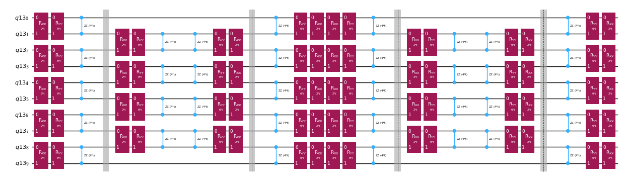
Au lieu d'implémenter l'opérateur d'évolution temporelle de manière exacte, nous pouvons utiliser la décomposition de Trotter pour en implémenter une approximation. Répéter plusieurs fois une décomposition de Trotter d'un certain ordre permet de réduire davantage l'erreur introduite par cette approximation. Dans ce qui suit, nous construisons directement l'implémentation de Trotter de la manière la plus efficace possible compte tenu du graphe d'interactions du hamiltonien considéré (interactions aux premiers voisins uniquement). En pratique, nous insérons des rotations de Pauli $R_{xx}$, $R_{yy}$, $R_{zz}$ avec des constantes de couplage $J_x,$ $J_y,$ et $J_z$ et un angle paramétré $t$, qui correspondent à l'implémentation approchée de $e^{-i (J_x XX + J_y YY + J_z ZZ) t}$. Étant donné la différence de définition entre les rotations de Pauli et l'évolution temporelle que nous cherchons à implémenter, nous devrons utiliser le paramètre $2*dt$ pour obtenir une évolution temporelle de $dt$. De plus, nous inversons l'ordre des opérations pour les répétitions en nombre impair des étapes de Trotter, ce qui est fonctionnellement équivalent mais permet de synthétiser des opérations adjacentes en un seul unitaire $SU(2)$. Cela donne un circuit bien moins profond que ce qu'on obtient avec la fonctionnalité générique PauliEvolutionGate().

t = Parameter("t")

# Create instruction for rotation about XX+YY-ZZ:
Rxyz_circ = QuantumCircuit(2)
Rxyz_circ.rxx(2 * JX * t, 0, 1)
Rxyz_circ.ryy(2 * JY * t, 0, 1)
Rxyz_circ.rzz(2 * JZ * t, 0, 1)
Rxyz_instr = Rxyz_circ.to_instruction(label="R J_x XX + J_y YY + J_z ZZ")

interaction_list = [
    [[i, i + 1] for i in range(0, n_qubits - 1, 2)],
    [[i, i + 1] for i in range(1, n_qubits - 1, 2)],
]  # linear chain

qr = QuantumRegister(n_qubits)
trotter_step_circ = QuantumCircuit(qr)
for i, color in enumerate(interaction_list):
    for interaction in color:
        trotter_step_circ.append(Rxyz_instr, interaction)
    if i < len(interaction_list) - 1:
        trotter_step_circ.barrier()
reverse_trotter_step_circ = trotter_step_circ.reverse_ops()

qc_evol = QuantumCircuit(qr)
for step in range(num_trotter_steps):
    if step % 2 == 0:
        qc_evol = qc_evol.compose(trotter_step_circ)
    else:
        qc_evol = qc_evol.compose(reverse_trotter_step_circ)

qc_evol.decompose().draw("mpl", fold=-1, scale=0.5)

Nous préparons à nouveau un état initial pour ce test de Hadamard efficace.

control = 0
excitation = int(n_qubits / 2) + 1
controlled_state_prep = QuantumCircuit(n_qubits + 1)
controlled_state_prep.cx(control, excitation)
controlled_state_prep.draw("mpl", fold=-1, scale=0.5)

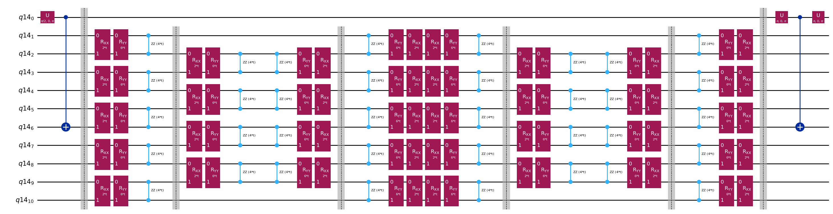
Circuits modèles pour le calcul des éléments de matrice de $\tilde{S}$ et $\tilde{H}$ via le test de Hadamard

La seule différence entre les circuits utilisés dans le test de Hadamard sera la phase dans l'opérateur d'évolution temporelle et les observables mesurées. Nous pouvons donc préparer un circuit modèle représentant le circuit générique pour le test de Hadamard, avec des emplacements réservés pour les portes qui dépendent de l'opérateur d'évolution temporelle.

# Parameters for the template circuits
parameters = []
for idx in range(1, krylov_dim):
    parameters.append(dt_circ * (idx))

# Create modified hadamard test circuit
qr = QuantumRegister(n_qubits + 1)
qc = QuantumCircuit(qr)
qc.h(0)
qc.compose(controlled_state_prep, list(range(n_qubits + 1)), inplace=True)
qc.barrier()
qc.compose(qc_evol, list(range(1, n_qubits + 1)), inplace=True)
qc.barrier()
qc.x(0)
qc.compose(controlled_state_prep.inverse(), list(range(n_qubits + 1)), inplace=True)
qc.x(0)

qc.decompose().draw("mpl", fold=-1)

print(
    "The optimized circuit has 2Q gates depth: ",
    qc.decompose().decompose().depth(lambda x: x[0].num_qubits == 2),
)

The optimized circuit has 2Q gates depth:  50

Cette profondeur est considérablement réduite par rapport au test de Hadamard d'origine. Elle reste gérable sur les ordinateurs quantiques modernes, bien qu'elle soit encore assez élevée. Nous devrons recourir à des techniques de mitigation d'erreurs de pointe pour obtenir des résultats exploitables.

Sélectionne un backend sur lequel exécuter notre calcul de Krylov quantique, afin de pouvoir transpiler notre circuit pour l'exécuter sur cet ordinateur quantique.

# Use the least-busy backend or specify a quantum computer using the syntax commented out below.
service = QiskitRuntimeService()
backend = service.least_busy(operational=True, simulator=False)

# Or you may choose a specify backend and channel if necessary for your workflow.
# service = QiskitRuntimeService(channel="ibm_quantum_platform")
# backend = service.backend("ibm_fez")

Nous transpilon maintenant nos circuits et opérateurs.

from qiskit.transpiler.preset_passmanagers import generate_preset_pass_manager

target = backend.target
basis_gates = list(target.operation_names)
pm = generate_preset_pass_manager(
    optimization_level=3, backend=backend, basis_gates=basis_gates
)

qc_trans = pm.run(qc)

print(qc_trans.depth(lambda x: x[0].num_qubits == 2))
print(qc_trans.count_ops())
qc_trans.draw("mpl", fold=-1, idle_wires=False, scale=0.5)

36
OrderedDict([('rz', 410), ('sx', 361), ('cz', 156), ('x', 18), ('barrier', 6)])

Après optimisation, la profondeur à deux qubits de notre circuit transpilé est encore réduite.

4.3 Étape 3. Exécuter avec une primitive Qiskit Runtime

Nous créons maintenant des PUBs pour l'exécution avec Estimator.

# Define observables to measure for S
observable_S_real = "I" * (n_qubits) + "X"
observable_S_imag = "I" * (n_qubits) + "Y"

observable_op_real = SparsePauliOp(
    observable_S_real
)  # define a sparse pauli operator for the observable
observable_op_imag = SparsePauliOp(observable_S_imag)

layout = qc_trans.layout  # get layout of transpiled circuit
observable_op_real = observable_op_real.apply_layout(
    layout
)  # apply physical layout to the observable
observable_op_imag = observable_op_imag.apply_layout(layout)
observable_S_real = (
    observable_op_real.paulis.to_labels()
)  # get the label of the physical observable
observable_S_imag = observable_op_imag.paulis.to_labels()

observables_S = [[observable_S_real], [observable_S_imag]]

# Define observables to measure for H
# Hamiltonian terms to measure
observable_list = []
for pauli, coeff in zip(H_op.paulis, H_op.coeffs):
    # print(pauli)
    observable_H_real = pauli[::-1].to_label() + "X"
    observable_H_imag = pauli[::-1].to_label() + "Y"
    observable_list.append([observable_H_real])
    observable_list.append([observable_H_imag])

layout = qc_trans.layout

observable_trans_list = []
for observable in observable_list:
    observable_op = SparsePauliOp(observable)
    observable_op = observable_op.apply_layout(layout)
    observable_trans_list.append([observable_op.paulis.to_labels()])

observables_H = observable_trans_list

# Define a sweep over parameter values
params = np.vstack(parameters).T

# Estimate the expectation value for all combinations of
# observables and parameter values, where the pub result will have
# shape (# observables, # parameter values).
pub = (qc_trans, observables_S + observables_H, params)

Les circuits pour $t=0$ sont calculables classiquement. Nous effectuons ce calcul avant de passer au cas $t\neq 0$ à l'aide d'un ordinateur quantique.

from qiskit.quantum_info import StabilizerState, Pauli

qc_cliff = qc.assign_parameters({t: 0})

# Get expectation values from experiment
S_expval_real = StabilizerState(qc_cliff).expectation_value(
    Pauli("I" * (n_qubits) + "X")
)
S_expval_imag = StabilizerState(qc_cliff).expectation_value(
    Pauli("I" * (n_qubits) + "Y")
)

# Get expectation values
S_expval = S_expval_real + 1j * S_expval_imag

H_expval = 0
for obs_idx, (pauli, coeff) in enumerate(zip(H_op.paulis, H_op.coeffs)):
    # Get expectation values from experiment
    expval_real = StabilizerState(qc_cliff).expectation_value(
        Pauli(pauli[::-1].to_label() + "X")
    )
    expval_imag = StabilizerState(qc_cliff).expectation_value(
        Pauli(pauli[::-1].to_label() + "Y")
    )
    expval = expval_real + 1j * expval_imag

    # Fill-in matrix elements
    H_expval += coeff * expval

print(H_expval)

(10+0j)

Bien que nous ayons réussi à réduire notre profondeur de portes d'ordres de grandeur grâce au test de Hadamard efficace, la profondeur reste suffisante pour nécessiter des techniques de mitigation d'erreurs de pointe. Ci-dessous, nous précisons les attributs de la mitigation utilisée. Toutes les méthodes employées sont importantes, mais il vaut la peine de mentionner spécifiquement l'amplification d'erreur probabiliste (PEA). Cette technique puissante s'accompagne d'un surcoût quantique considérable. Le calcul effectué ici peut prendre 20 minutes ou plus sur un vrai ordinateur quantique. Tu peux jouer avec les paramètres ci-dessous pour augmenter ou réduire la précision et, par conséquent, le surcoût. Les paramètres par défaut ci-dessous donnent des résultats de haute fidélité.

# Experiment options
num_randomizations = 300
num_randomizations_learning = 20
max_batch_circuits = 20
shots_per_randomization = 100
learning_pair_depths = [0, 4, 24]
noise_factors = [1, 1.3, 1.6]

# Base option formatting
options = {
    # Builtin resilience settings for ZNE
    "resilience": {
        "measure_mitigation": True,
        "zne_mitigation": True,
        "zne": {"noise_factors": noise_factors},
        # TREX noise learning configuration
        "measure_noise_learning": {
            "num_randomizations": num_randomizations_learning,
            "shots_per_randomization": shots_per_randomization,
        },
        # PEA noise model configuration
        "layer_noise_learning": {
            "max_layers_to_learn": 10,
            "layer_pair_depths": learning_pair_depths,
            "shots_per_randomization": shots_per_randomization,
            "num_randomizations": num_randomizations_learning,
        },
    },
    # Randomization configuration
    "twirling": {
        "num_randomizations": num_randomizations,
        "shots_per_randomization": shots_per_randomization,
        "strategy": "all",
    },
    # Experimental settings for PEA method
    "experimental": {
        # # Just in case, disable any further qiskit transpilation not related to twirling / DD
        # "skip_transpilation": True,
        # Execution configuration
        "execution": {
            "max_pubs_per_batch_job": max_batch_circuits,
            "fast_parametric_update": True,
        },
        # Error Mitigation configuration
        "resilience": {
            # ZNE Configuration
            "zne": {
                "amplifier": "pea",
                "return_all_extrapolated": True,
                "return_unextrapolated": True,
                "extrapolated_noise_factors": [0] + noise_factors,
            }
        },
    },
}

Enfin, nous exécutons les circuits pour $\tilde{S}$ et $\tilde{H}$ avec Estimator.

# This job required 17 minutes of QPU time to run on a Heron r2 processor. This is only an estimate.
# Your execution time may vary.

with Batch(backend=backend) as batch:
    # Estimator
    estimator = Estimator(mode=batch, options=options)

    job = estimator.run([pub], precision=1)

4.4 Étape 4. Post-traitement et analyse des résultats

Ce que nous avons obtenu de l'ordinateur quantique, ce sont les éléments de matrice individuels de $\tilde{S}$ et les groupes de Pauli qui commutent et constituent les éléments de matrice de $\tilde{H}$. Ces termes doivent être combinés pour retrouver nos matrices, afin de pouvoir résoudre le problème aux valeurs propres généralisé.

# Store the outputs as 'results'.
results = job.result()[0]

Calculer le hamiltonien effectif et les matrices de recouvrement

Calcule d'abord la phase accumulée par l'état $\vert 0 \rangle$ lors de l'évolution temporelle non contrôlée.

prefactors = [
    np.exp(-1j * sum([c for p, c in H_op.to_list() if "Z" in p]) * i * dt)
    for i in range(1, krylov_dim)
]

Une fois les résultats des exécutions de circuits obtenus, nous pouvons post-traiter les données pour calculer les éléments de matrice de $S$

# Assemble S, the overlap matrix of dimension D:
S_first_row = np.zeros(krylov_dim, dtype=complex)
S_first_row[0] = 1 + 0j

# Add in ancilla-only measurements:
for i in range(krylov_dim - 1):
    # Get expectation values from experiment
    expval_real = results.data.evs[0][0][i]  # automatic extrapolated evs if ZNE is used
    expval_imag = results.data.evs[1][0][i]  # automatic extrapolated evs if ZNE is used

    # Get expectation values
    expval = expval_real + 1j * expval_imag
    S_first_row[i + 1] += prefactors[i] * expval

S_first_row_list = S_first_row.tolist()  # for saving purposes

S_circ = np.zeros((krylov_dim, krylov_dim), dtype=complex)

# Distribute entries from first row across matrix:
for i, j in it.product(range(krylov_dim), repeat=2):
    if i >= j:
        S_circ[j, i] = S_first_row[i - j]
    else:
        S_circ[j, i] = np.conj(S_first_row[j - i])

from sympy import Matrix

Matrix(S_circ)

$$\displaystyle \left[\begin{matrix}1.0 & 0.149322296177984 - 0.283023058106896 i & 0.185815978760175 - 0.0910521940394691 i & 0.0940509850777074 - 0.094154537369141 i\\0.149322296177984 + 0.283023058106896 i & 1.0 & 0.149322296177984 - 0.283023058106896 i & 0.185815978760175 - 0.0910521940394691 i\\0.185815978760175 + 0.0910521940394691 i & 0.149322296177984 + 0.283023058106896 i & 1.0 & 0.149322296177984 - 0.283023058106896 i\\0.0940509850777074 + 0.094154537369141 i & 0.185815978760175 + 0.0910521940394691 i & 0.149322296177984 + 0.283023058106896 i & 1.0\end{matrix}\right]$$

Et les éléments de matrice de $\tilde{H}$

import itertools

# Assemble S, the overlap matrix of dimension D:
H_first_row = np.zeros(krylov_dim, dtype=complex)
H_first_row[0] = H_expval

for obs_idx, (pauli, coeff) in enumerate(zip(H_op.paulis, H_op.coeffs)):
    # Add in ancilla-only measurements:
    for i in range(krylov_dim - 1):
        # Get expectation values from experiment
        expval_real = results.data.evs[2 + 2 * obs_idx][0][
            i
        ]  # automatic extrapolated evs if ZNE is used
        expval_imag = results.data.evs[2 + 2 * obs_idx + 1][0][
            i
        ]  # automatic extrapolated evs if ZNE is used

        # Get expectation values
        expval = expval_real + 1j * expval_imag
        H_first_row[i + 1] += prefactors[i] * coeff * expval

H_first_row_list = H_first_row.tolist()

H_eff_circ = np.zeros((krylov_dim, krylov_dim), dtype=complex)

# Distribute entries from first row across matrix:
for i, j in itertools.product(range(krylov_dim), repeat=2):
    if i >= j:
        H_eff_circ[j, i] = H_first_row[i - j]
    else:
        H_eff_circ[j, i] = np.conj(H_first_row[j - i])

from sympy import Matrix

Matrix(H_eff_circ)

$$\displaystyle \left[\begin{matrix}10.0 & -3.02044405310714 - 2.80721615865252 i & 0.496487054782717 + 0.188101957039621 i & 1.0770511571923 + 0.104340737159455 i\\-3.02044405310714 + 2.80721615865252 i & 10.0 & -3.02044405310714 - 2.80721615865252 i & 0.496487054782717 + 0.188101957039621 i\\0.496487054782717 - 0.188101957039621 i & -3.02044405310714 + 2.80721615865252 i & 10.0 & -3.02044405310714 - 2.80721615865252 i\\1.0770511571923 - 0.104340737159455 i & 0.496487054782717 - 0.188101957039621 i & -3.02044405310714 + 2.80721615865252 i & 10.0\end{matrix}\right]$$

Enfin, nous pouvons résoudre le problème aux valeurs propres généralisé pour $\tilde{H}$ :

$\tilde{H} \vec{c} = c S \vec{c}$

et obtenir une estimation de l'énergie de l'état fondamental $c_{min}$

gnd_en_circ_est_list = []
for d in range(1, krylov_dim + 1):
    # Solve generalized eigenvalue problem
    gnd_en_circ_est = solve_regularized_gen_eig(
        H_eff_circ[:d, :d], S_circ[:d, :d], threshold=1e-1
    )
    gnd_en_circ_est_list.append(gnd_en_circ_est)
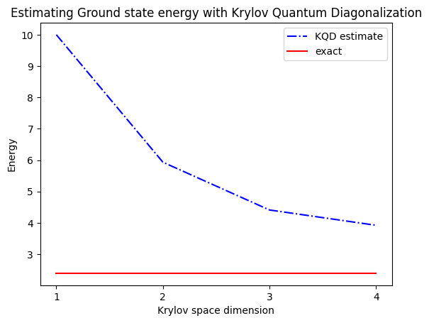
    print("The estimated ground state energy is: ", gnd_en_circ_est)

The estimated ground state energy is:  10.0
The estimated ground state energy is:  5.933953916292923
The estimated ground state energy is:  4.4101773995740645
The estimated ground state energy is:  3.921288588521255

Pour un secteur à une seule particule, nous pouvons calculer efficacement l'état fondamental de ce secteur du hamiltonien de manière classique.

gs_en = single_particle_gs(H_op, n_qubits)

n_sys_qubits 10
n_exc 1 , subspace dimension 11
single particle ground state energy:  2.391547869638771

len(H_op)

27

plt.plot(
    range(1, krylov_dim + 1),
    gnd_en_circ_est_list,
    color="blue",
    linestyle="-.",
    label="KQD estimate",
)
plt.plot(
    range(1, krylov_dim + 1),
    [gs_en] * krylov_dim,
    color="red",
    linestyle="-",
    label="exact",
)
plt.xticks(range(1, krylov_dim + 1), range(1, krylov_dim + 1))
plt.legend()
plt.xlabel("Krylov space dimension")
plt.ylabel("Energy")
plt.title("Estimating Ground state energy with Krylov Quantum Diagonalization")
plt.show()

5. Discussion et extension

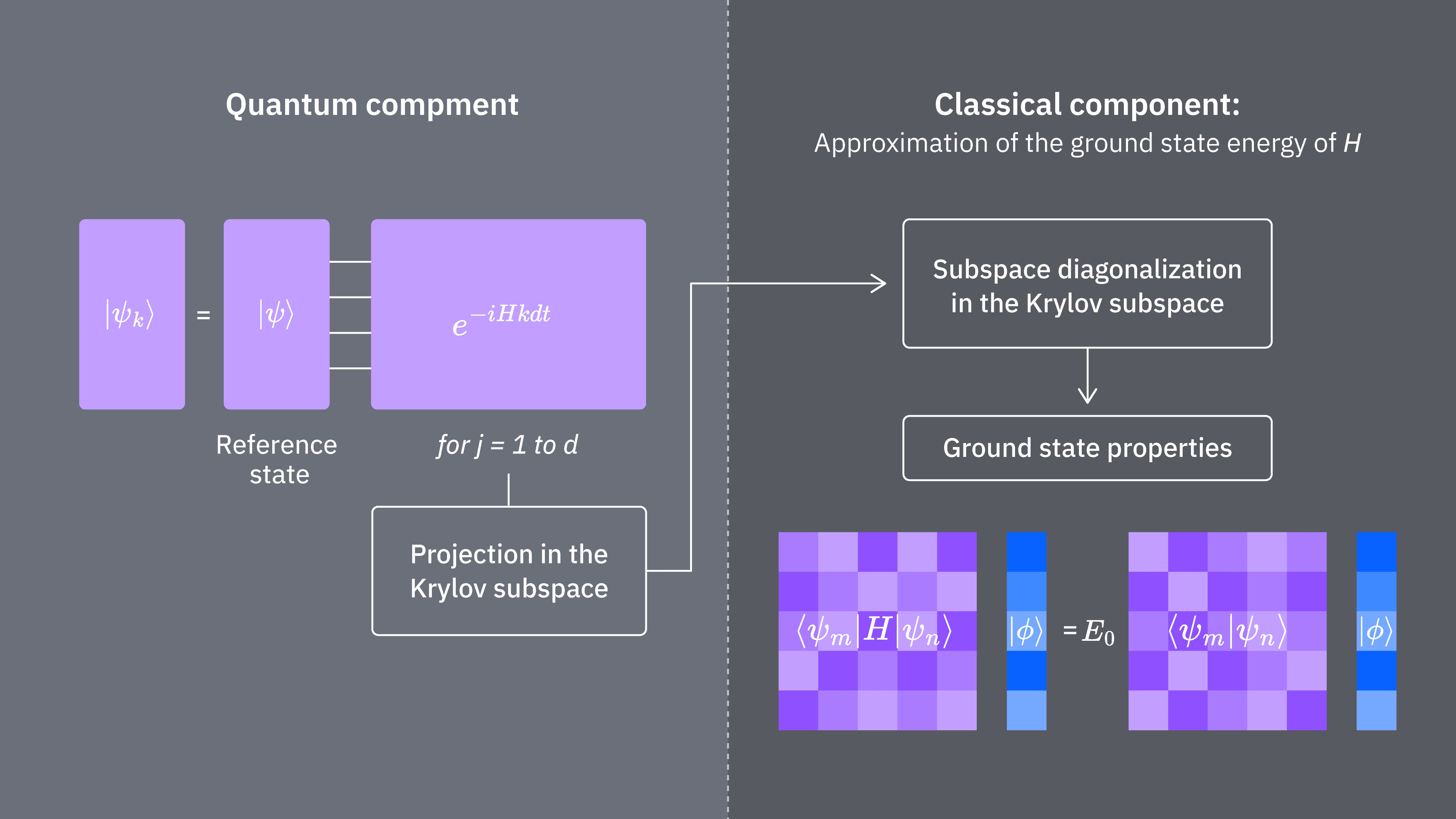
Pour récapituler, on part d'un état de référence, puis on le fait évoluer pendant différentes durées pour générer le sous-espace de Krylov unitaire. On projette notre hamiltonien sur ce sous-espace. On estime également les recouvrements des vecteurs du sous-espace. Enfin, on résout classiquement le problème aux valeurs propres généralisé de dimension réduite.

Comparons ce qui détermine les coûts de calcul lors de l'utilisation de la technique de Krylov de manière classique et quantique. Il n'existe pas d'analogies parfaites entre les approches classique et quantique pour toutes les étapes. Ce tableau rassemble quelques informations sur la mise à l'échelle de différentes étapes pour comparaison.

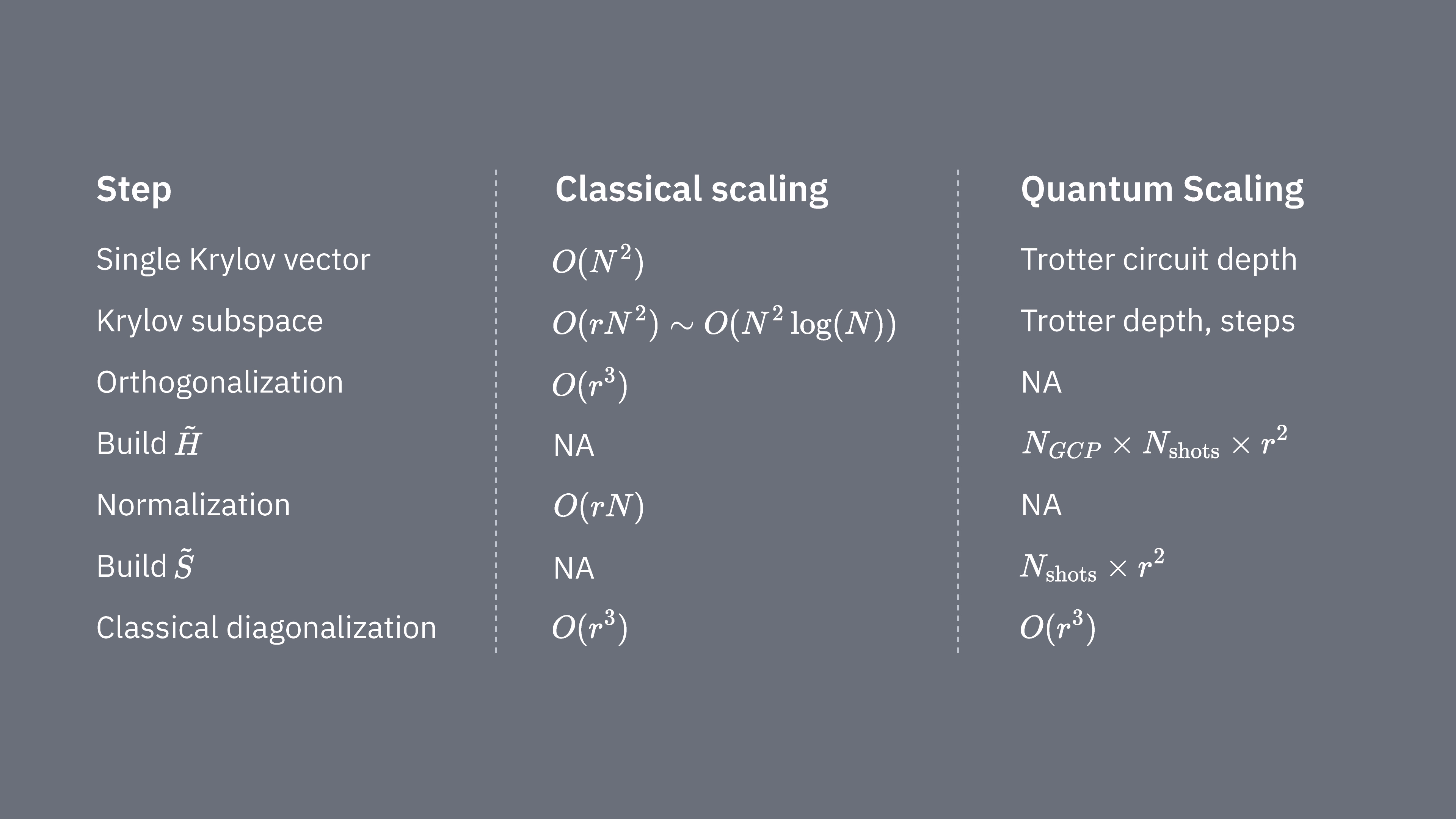
Rappelle-toi que les hamiltoniens ont généralement des termes qui ne peuvent pas être mesurés simultanément (parce qu'ils ne commutent pas entre eux). On trie les termes du hamiltonien en groupes d'opérateurs de Pauli commutatifs qui peuvent tous être mesurés simultanément, et on peut avoir besoin de nombreux groupes de ce type pour prendre en compte tous les termes qui ne commutent pas entre eux. Pour construire $\tilde{H}$ sur un ordinateur quantique, il faut effectuer des mesures séparées pour chaque groupe de chaînes de Pauli commutatives dans le hamiltonien, et chacune d'elles nécessite de nombreux shots. On doit faire cela pour $r^2$ éléments de matrice différents, correspondant à $r^2$ combinaisons de différents facteurs d'évolution temporelle. Il existe parfois des moyens de réduire cela, mais dans ce traitement approximatif, le temps nécessaire pour cela évolue comme $N_\text{shots}\times N_\text{GCP} \times r^2.$ Les éléments de $S$ doivent être estimés, ce qui évolue comme $O(N_\text{shots}\times r^2)$. Enfin, la résolution du problème aux valeurs propres généralisé dans l'espace projeté, de façon classique, prend $O(r^3).$

On voit que la diagonalisation quantique de Krylov peut être utile dans les cas où le nombre de groupes de Pauli commutatifs dans le hamiltonien est relativement faible. Ces dépendances de mise à l'échelle suggèrent certaines applications où la méthode de Krylov peut être utile, et d'autres où elle ne le sera probablement pas. Certains hamiltoniens ont une grande complexité lorsqu'ils sont mappés sur des qubits, impliquant de nombreuses chaînes de Pauli non commutatives qui ne peuvent pas facilement être partitionnées en quelques groupes commutatifs. C'est souvent le cas des problèmes de chimie quantique, par exemple. Cette complexité présente deux défis principaux pour les ordinateurs quantiques à court terme :

• L'estimation de chaque élément de $\tilde{H}$ devient coûteuse en calcul en raison du grand nombre de termes.
• Les circuits de Trotter nécessaires deviennent trop profonds pour être utilisables.

Ces deux points ci-dessus seront moins problématiques lorsque les ordinateurs quantiques atteindront la tolérance aux fautes, mais ils doivent être pris en compte à court terme. Même les systèmes avec des mappages « plus simples » que ceux de la chimie quantique peuvent rencontrer les mêmes obstacles, si les hamiltoniens ont trop de termes non commutatifs. La méthode de Krylov est la plus utile lorsque le hamiltonien peut être partitionné en relativement peu de groupes de Pauli commutatifs, et lorsque $H$ est facile à implémenter dans des circuits de Trotter. Ces deux conditions sont satisfaites, par exemple, pour de nombreux modèles de réseau d'intérêt en physique. KQD est particulièrement utile lorsqu'on sait très peu de chose sur l'état fondamental. Cela découle de ses garanties de convergence inhérentes et de son applicabilité dans des scénarios où des méthodes alternatives sont inapplicables en raison d'une connaissance insuffisante de l'état fondamental.

Bien que KQD soit un outil puissant, les aspects chronophages du protocole, notamment l'estimation de chaque élément du hamiltonien projeté et le recouvrement des états de Krylov, représentent des opportunités d'amélioration. Une approche alternative consiste à exploiter les méthodes de Krylov en conjonction avec des méthodes basées sur l'échantillonnage, qui font l'objet de la prochaine leçon.

6. Appendices

Annexe I : sous-espace de Krylov à partir d'évolutions temporelles réelles

L'espace de Krylov unitaire est défini comme

$$\mathcal{K}_U(H, |\psi\rangle) = \text{span}\left\{ |\psi\rangle, e^{-iH\,dt} |\psi\rangle, \dots, e^{-irH\,dt} |\psi\rangle \right\}$$

pour un certain pas de temps $dt$ que nous allons déterminer plus tard. Supposons temporairement que $r$ soit pair : définissons alors $d=r/2$. Remarque que lorsqu'on projette le hamiltonien dans le sous-espace de Krylov ci-dessus, il est impossible de le distinguer du sous-espace de Krylov

$$\mathcal{K}_U(H, |\psi\rangle) = \text{span}\left\{ e^{i\,d\,H\,dt}|\psi\rangle, e^{i(d-1)H\,dt} |\psi\rangle, \dots, e^{-i(d-1)H\,dt} |\psi\rangle, e^{-i\,d\,H\,dt} |\psi\rangle \right\},$$

c'est-à-dire celui où toutes les évolutions temporelles sont décalées en arrière de $d$ pas de temps. La raison pour laquelle il est impossible de les distinguer est que les éléments de matrice

$$\tilde{H}_{j,k} = \langle\psi|e^{i\,j\,H\,dt}He^{-i\,k\,H\,dt}|\psi\rangle=\langle\psi|He^{i(j-k)H\,dt}|\psi\rangle$$

sont invariants sous des décalages globaux du temps d'évolution, puisque les évolutions temporelles commutent avec le hamiltonien. Pour $r$ impair, on peut utiliser l'analyse pour $r-1$.

On veut montrer que quelque part dans cet espace de Krylov, il est garanti qu'il existe un état de basse énergie. Pour ce faire, on s'appuie sur le résultat suivant, qui est dérivé du Théorème 3.1 dans [3] :

Affirmation 1 : il existe une fonction $f$ telle que pour les énergies $E$ dans la plage spectrale du hamiltonien (c'est-à-dire entre l'énergie de l'état fondamental et l'énergie maximale)…

1. $f(E_0)=1$
2. $|f(E)|\le2\left(1 + \delta\right)^{-d}$ pour toutes les valeurs de $E$ qui se trouvent à $\ge\delta$ de $E_0$, c'est-à-dire qu'elle est exponentiellement supprimée
3. $f(E)$ est une combinaison linéaire de $e^{ijE\,dt}$ pour $j=-d,-d+1,...,d-1,d$

On donne une preuve ci-dessous, mais elle peut être ignorée sans problème à moins qu'on ne veuille comprendre l'argument rigoureux complet. Pour l'instant, concentrons-nous sur les implications de l'affirmation ci-dessus. Par la propriété 3 ci-dessus, on peut voir que l'espace de Krylov décalé ci-dessus contient l'état $f(H)|\psi\rangle$. C'est notre état de basse énergie. Pour comprendre pourquoi, on écrit $|\psi\rangle$ dans la base des états propres d'énergie :

$$|\psi\rangle = \sum_{k=0}^{N}\gamma_k|E_k\rangle,$$

où $|E_k\rangle$ est le k-ième état propre d'énergie et $\gamma_k$ est son amplitude dans l'état initial $|\psi\rangle$. Exprimé en ces termes, $f(H)|\psi\rangle$ est donné par

$$f(H)|\psi\rangle = \sum_{k=0}^{N}\gamma_kf(E_k)|E_k\rangle,$$

en utilisant le fait qu'on peut remplacer $H$ par $E_k$ lorsqu'il agit sur l'état propre $|E_k\rangle$. L'erreur d'énergie de cet état est donc

$$\text{erreur d'énergie} = \frac{\langle\psi|f(H)(H-E_0)f(H)|\psi\rangle}{\langle\psi|f(H)^2|\psi\rangle}$$ $$= \frac{\sum_{k=0}^{N}|\gamma_k|^2f(E_k)^2(E_k-E_0)}{\sum_{k=0}^{N}|\gamma_k|^2f(E_k)^2}.$$

Pour transformer cela en une borne supérieure plus facile à comprendre, on sépare d'abord la somme dans le numérateur entre les termes avec $E_k-E_0\le\delta$ et les termes avec $E_k-E_0>\delta$ :

$$\text{erreur d'énergie} = \frac{\sum_{E_k\le E_0+\delta}|\gamma_k|^2f(E_k)^2(E_k-E_0)}{\sum_{k=0}^{N}|\gamma_k|^2f(E_k)^2} + \frac{\sum_{E_k> E_0+\delta}|\gamma_k|^2f(E_k)^2(E_k-E_0)}{\sum_{k=0}^{N}|\gamma_k|^2f(E_k)^2}.$$

On peut borner supérieurement le premier terme par $\delta$,

$$\frac{\sum_{E_k\le E_0+\delta}|\gamma_k|^2f(E_k)^2(E_k-E_0)}{\sum_{k=0}^{N}|\gamma_k|^2f(E_k)^2} < \frac{\delta\sum_{E_k\le E_0+\delta}|\gamma_k|^2f(E_k)^2}{\sum_{k=0}^{N}|\gamma_k|^2f(E_k)^2} \le \delta,$$

où la première étape découle du fait que $E_k-E_0\le\delta$ pour chaque $E_k$ dans la somme, et la deuxième étape découle du fait que la somme au numérateur est un sous-ensemble de la somme au dénominateur. Pour le deuxième terme, on borne d'abord inférieurement le dénominateur par $|\gamma_0|^2$, puisque $f(E_0)^2=1$ : en rassemblant tout, on obtient

$$\text{erreur d'énergie} \le \delta + \frac{1}{|\gamma_0|^2}\sum_{E_k>E_0+\delta}|\gamma_k|^2f(E_k)^2(E_k-E_0).$$

Pour simplifier ce qui reste, remarque que pour tous ces $E_k$, par la définition de $f$ on sait que $f(E_k)^2 \le 4\left(1 + \delta\right)^{-2d}$. En bornant supérieurement $E_k-E_0<2\|H\|$ et en bornant supérieurement $\sum_{E_k>E_0+\delta}|\gamma_k|^2<1$, on obtient

$$\text{erreur d'énergie} \le \delta + \frac{8}{|\gamma_0|^2}\|H\|\left(1 + \delta\right)^{-2d}.$$

Cela est valable pour tout $\delta>0$, donc si on fixe $\delta$ égal à notre erreur cible, alors la borne d'erreur ci-dessus converge vers celle-ci exponentiellement avec la dimension de Krylov $2d=r$. Remarque également que si $\delta<E_1-E_0$, alors le terme $\delta$ disparaît complètement dans la borne ci-dessus.

Pour compléter l'argument, on note d'abord que ce qui précède n'est que l'erreur d'énergie de l'état particulier $f(H)|\psi\rangle$, plutôt que l'erreur d'énergie de l'état de plus basse énergie dans l'espace de Krylov. Cependant, par le principe variationnel (Rayleigh-Ritz), l'erreur d'énergie de l'état de plus basse énergie dans l'espace de Krylov est bornée supérieurement par l'erreur d'énergie de n'importe quel état dans l'espace de Krylov, donc ce qui précède est également une borne supérieure sur l'erreur d'énergie de l'état de plus basse énergie, c'est-à-dire la sortie de l'algorithme de diagonalisation quantique de Krylov.

Une analyse similaire à celle ci-dessus peut être menée qui prend également en compte le bruit et la procédure de seuillage discutée dans le notebook. Voir [2] et [4] pour cette analyse.

Annexe II : preuve de l'Affirmation 1

Ce qui suit est principalement dérivé de [3], Théorème 3.1 : soient $0 < a < b$ et $\Pi^*_d$ l'espace des polynômes résiduels (polynômes dont la valeur en 0 est 1) de degré au plus $d$. La solution de

$$\beta(a, b, d) = \min_{p \in \Pi^*_d} \max_{x \in [a, b]} |p(x)| \quad$$

est

$$p^*(x) = \frac{T_d\left(\frac{b + a - 2x}{b - a}\right)}{T_d\left(\frac{b + a}{b - a}\right)}, \quad$$

et la valeur minimale correspondante est

$$\beta(a, b, d) = T_d^{-1}\left(\frac{b + a}{b - a}\right).$$

On veut convertir cela en une fonction qui peut être exprimée naturellement en termes d'exponentielles complexes, parce que ce sont les évolutions temporelles réelles qui génèrent l'espace de Krylov quantique. Pour ce faire, il est commode d'introduire la transformation suivante des énergies dans la plage spectrale du hamiltonien vers des nombres dans la plage $[0,1]$ : définissons

$$g(E) = \frac{1-\cos\big((E-E_0)dt\big)}{2},$$

où $dt$ est un pas de temps tel que $-\pi < E_0dt < E_\text{max}dt < \pi$. Remarque que $g(E_0)=0$ et que $g(E)$ croît à mesure que $E$ s'éloigne de $E_0$.

En utilisant maintenant le polynôme $p^*(x)$ avec les paramètres a, b, d fixés à $a = g(E_0 + \delta)$, $b = 1$, et d = int(r/2), on définit la fonction :

$$f(E) = p^* \left( g(E) \right) = \frac{T_d\left(1 + 2\frac{\cos\big((E-E_0)dt\big) - \cos\big(\delta\,dt\big)}{1 +\cos\big(\delta\,dt\big)}\right)}{T_d\left(1 + 2\frac{1-\cos\big(\delta\,dt\big)}{1 + \cos\big(\delta\,dt\big)}\right)}$$

où $E_0$ est l'énergie de l'état fondamental. On peut voir en insérant $\cos(x)=\frac{e^{ix}+e^{-ix}}{2}$ que $f(E)$ est un polynôme trigonométrique de degré $d$, c'est-à-dire une combinaison linéaire de $e^{ijE\,dt}$ pour $j=-d,-d+1,...,d-1,d$. De plus, à partir de la définition de $p^*(x)$ ci-dessus, on a que $f(E_0)=p(0)=1$ et pour tout $E$ dans la plage spectrale tel que $\vert E-E_0 \vert > \delta$, on a

$$|f(E)| \le \beta(a, b, d) = T_d^{-1}\left(1 + 2\frac{1-\cos\big(\delta\,dt\big)}{1 + \cos\big(\delta\,dt\big)}\right)$$ $$\leq 2\left(1 + \delta\right)^{-d} = 2\left(1 + \delta\right)^{-\lfloor k/2\rfloor}.$$

Références :

[1] https://arxiv.org/abs/2407.14431

[2] https://arxiv.org/abs/1811.09025

[3] https://people.math.ethz.ch/~mhg/pub/biksm.pdf

[4] https://academic.oup.com/book/36426

[5] https://en.wikipedia.org/wiki/Krylov_subspace

[6] Krylov Subspace Methods: Principles and Analysis, Jörg Liesen, Zdenek Strakos https://academic.oup.com/book/36426

[7] Iterative Methods for Sparse Linear Systems" by Yousef Saad

[8] "MINRES-QLP: A Krylov Subspace Method for Indefinite or Singular Symmetric Systems" by Sou-Cheng Choi, Christopher Paige, and Michael Saunders (https://epubs.siam.org/doi/10.1137/100787921)

[9] Ethan N. Epperly, Lin Lin, and Yuji Nakatsukasa. "A theory of quantum subspace diagonalization". SIAM Journal on Matrix Analysis and Applications 43, 1263–1290 (2022).