Le solveur propre quantique variationnel (VQE)

Cette leçon présente le solveur propre quantique variationnel, explique son importance en tant qu'algorithme fondateur en informatique quantique, et explore ses forces et ses faiblesses. Le VQE seul, sans méthodes complémentaires, ne suffit probablement pas pour des calculs quantiques à l'échelle utilitaire moderne. Il reste néanmoins essentiel en tant qu'exemple archétypal de méthode hybride classique-quantique, et constitue une base importante sur laquelle reposent de nombreux algorithmes plus avancés.

Cette vidéo donne un aperçu du VQE et des facteurs qui influencent son efficacité. Le texte ci-dessous apporte plus de détails et implémente le VQE avec Qiskit.

1. Qu'est-ce que le VQE ?

Le solveur propre quantique variationnel est un algorithme qui utilise conjointement le calcul classique et quantique pour accomplir une tâche. Un calcul VQE repose sur 4 composantes principales :

Un opérateur : souvent un Hamiltonien, que l'on notera $H$ , qui décrit une propriété du système que l'on souhaite optimiser. Autrement dit, on cherche le vecteur propre de cet opérateur correspondant à la valeur propre minimale. On appelle souvent ce vecteur propre l'« état fondamental ».
Un « ansatz » (mot allemand signifiant « approche ») : il s'agit d'un circuit quantique qui prépare un état quantique approximant le vecteur propre recherché. L'ansatz est en réalité une famille de circuits quantiques, car certaines portes de l'ansatz sont paramétrées, c'est-à-dire qu'elles reçoivent un paramètre que l'on peut faire varier. Cette famille de circuits quantiques peut préparer une famille d'états quantiques approchant l'état fondamental.
Un estimateur : un moyen d'estimer la valeur d'espérance de l'opérateur $H$ pour l'état quantique variationnel courant. Parfois, ce qui nous intéresse vraiment, c'est simplement cette valeur d'espérance, que l'on appelle fonction de coût. Parfois, on s'intéresse à une fonction plus complexe qui peut tout de même s'écrire à partir d'une ou plusieurs valeurs d'espérance.
Un optimiseur classique : un algorithme qui fait varier les paramètres pour tenter de minimiser la fonction de coût.

Examinons chacune de ces composantes plus en détail.

1.1 L'opérateur (Hamiltonien)

Au cœur d'un problème VQE se trouve un opérateur qui décrit un système d'intérêt. On suppose ici que la valeur propre la plus basse et le vecteur propre correspondant de cet opérateur sont utiles à des fins scientifiques ou pratiques. Parmi les exemples, on peut citer un Hamiltonien chimique décrivant une molécule, dont la valeur propre la plus basse correspond à l'énergie de l'état fondamental de la molécule, et dont l'état propre correspondant décrit la géométrie ou la configuration électronique de la molécule. L'opérateur peut également décrire le coût d'un certain processus à optimiser, et les états propres peuvent correspondre à des routes ou des pratiques. Dans certains domaines comme la physique, un « Hamiltonien » désigne presque toujours un opérateur décrivant l'énergie d'un système physique. Mais en informatique quantique, il est courant de voir des opérateurs quantiques décrivant un problème d'entreprise ou logistique également appelés « Hamiltonien ». Nous adoptons cette convention ici.

Une image d'orbitales atomiques et une image d'un réseau composé de nombreux nœuds et connexions.

Mapper un problème physique ou d'optimisation sur des qubits est généralement une tâche non triviale, mais ces détails ne sont pas l'objet de ce cours. Une discussion générale sur le mappage d'un problème vers un opérateur quantique se trouve dans L'informatique quantique en pratique. Un examen plus approfondi du mappage de problèmes de chimie en opérateurs quantiques est disponible dans La chimie quantique avec VQE.

Pour les besoins de ce cours, on suppose que la forme du Hamiltonien est connue. Par exemple, un Hamiltonien pour une molécule d'hydrogène simple (sous certaines hypothèses d'espace actif, et en utilisant le mappeur de Jordan-Wigner) est :

# Added by doQumentation — required packages for this notebook
!pip install -q matplotlib numpy qiskit qiskit-ibm-runtime scipy

from qiskit.quantum_info import SparsePauliOp

hamiltonian = SparsePauliOp(
    [
        "IIII",
        "IIIZ",
        "IZII",
        "IIZI",
        "ZIII",
        "IZIZ",
        "IIZZ",
        "ZIIZ",
        "IZZI",
        "ZZII",
        "ZIZI",
        "YYYY",
        "XXYY",
        "YYXX",
        "XXXX",
    ],
    coeffs=[
        -0.09820182 + 0.0j,
        -0.1740751 + 0.0j,
        -0.1740751 + 0.0j,
        0.2242933 + 0.0j,
        0.2242933 + 0.0j,
        0.16891402 + 0.0j,
        0.1210099 + 0.0j,
        0.16631441 + 0.0j,
        0.16631441 + 0.0j,
        0.1210099 + 0.0j,
        0.17504456 + 0.0j,
        0.04530451 + 0.0j,
        0.04530451 + 0.0j,
        0.04530451 + 0.0j,
        0.04530451 + 0.0j,
    ],
)

Note que dans le Hamiltonien ci-dessus, il y a des termes comme ZZII et YYYY qui ne commutent pas entre eux. C'est-à-dire que pour évaluer ZZII, on doit mesurer l'opérateur de Pauli Z sur le qubit 3 (entre autres mesures). Mais pour évaluer YYYY, on doit mesurer l'opérateur de Pauli Y sur ce même qubit, le qubit 3. Il existe une relation d'incertitude entre les opérateurs Y et Z sur le même qubit ; on ne peut pas mesurer ces deux opérateurs en même temps. Nous reviendrons sur ce point ci-dessous, et tout au long du cours. Le Hamiltonien ci-dessus est un opérateur matriciel de taille $16\times 16$ . Diagonaliser l'opérateur pour trouver sa valeur propre d'énergie la plus basse n'est pas difficile.

import numpy as np

A = np.array(hamiltonian)
eigenvalues, eigenvectors = np.linalg.eigh(A)
print("The ground state energy is ", min(eigenvalues), "hartrees")

The ground state energy is  -1.1459778447627311 hartrees

Les solveurs propres classiques par force brute ne peuvent pas monter en charge pour décrire les énergies ou les géométries de très grands systèmes atomiques, comme des médicaments ou des protéines. Le VQE est l'une des premières tentatives d'exploiter l'informatique quantique pour ce problème.

Nous rencontrerons dans cette leçon des Hamiltoniens bien plus grands que celui ci-dessus. Mais il serait prématuré de pousser les limites de ce que le VQE peut faire, avant d'introduire quelques-uns des outils plus avancés qui peuvent compléter ou remplacer le VQE, plus loin dans ce cours.

1.2 Ansatz

Le mot « ansatz » est allemand et signifie « approche ». Le pluriel correct en allemand est « ansätze », bien que l'on rencontre souvent « ansatzes » ou « ansatze ». Dans le contexte du VQE, un ansatz est le circuit quantique utilisé pour créer une fonction d'onde multi-qubit qui approxime au mieux l'état fondamental du système étudié, et qui produit ainsi la valeur d'espérance la plus basse de l'opérateur. Ce circuit quantique contiendra des paramètres variationnels (souvent regroupés dans le vecteur de variables $\vec{\theta}$ ).

Une image d'un circuit quantique avec des paramètres variationnels étiquetés « theta ».

Un ensemble initial de valeurs $\vec{\theta_0}$ des paramètres variationnels est choisi. On appellera l'opération unitaire de l'ansatz sur le circuit $U_{\text{var}}(\vec{\theta_0})$ . Par défaut, tous les qubits des ordinateurs quantiques IBM® sont initialisés à l'état $|0\rangle$ . Lorsque le circuit est exécuté, l'état des qubits sera

|\psi(\vec{\theta_0})\rangle=U_{\text{var}}(\vec{\theta_0})|0\rangle^{\otimes N}

Si tout ce dont on avait besoin était l'énergie la plus basse (en utilisant le langage des systèmes physiques), on pourrait l'estimer en mesurant l'énergie de nombreuses fois et en prenant la plus basse. Mais on veut généralement aussi connaître la configuration qui donne cette énergie ou valeur propre minimale. L'étape suivante consiste donc à estimer la valeur d'espérance du Hamiltonien, ce qui s'effectue via des mesures quantiques. Cela implique beaucoup de choses. Mais on peut comprendre ce processus qualitativement en notant que la probabilité $P_j$ de mesurer une énergie $E_j$ (toujours en utilisant le langage des systèmes physiques) est liée à la valeur d'espérance par :

\langle \psi(\vec{\theta_0}) |H|\psi (\vec{\theta_0}) \rangle

La probabilité $P_j$ est également liée au recouvrement entre l'état propre $|\phi_j\rangle$ et l'état courant du système $|\psi(\vec{\theta_0})\rangle$ :

P_j=|\langle \phi_j|\psi(\vec{\theta_0})\rangle|^2 = |\langle \phi_j|U_{\text{var}}(\vec{\theta_0})|0\rangle^{\otimes N}|^2

Ainsi, en effectuant de nombreuses mesures des opérateurs de Pauli constituant notre Hamiltonien, on peut estimer la valeur d'espérance du Hamiltonien dans l'état courant du système $|\psi(\vec{\theta_0})\rangle$ . L'étape suivante consiste à faire varier les paramètres $\vec{\theta}$ et à tenter de se rapprocher davantage de l'état fondamental (de plus basse énergie) du système. Du fait des paramètres variationnels dans l'ansatz, on entend parfois parler de forme variationnelle.

Avant de passer à ce processus variationnel, note qu'il est souvent utile de démarrer depuis un état « proche de la solution ». Si tu connais suffisamment bien ton système, tu peux faire une meilleure supposition initiale que $|0\rangle^{\otimes N}$ . Par exemple, il est courant d'initialiser les qubits à l'état de Hartree-Fock dans les applications chimiques. Cet état de départ, qui ne contient aucun paramètre variationnel, est appelé l'état de référence. Notons $U_{ref}$ le circuit quantique utilisé pour créer l'état de référence. Lorsqu'il devient important de distinguer l'état de référence du reste de l'ansatz, on utilise : $U_{\text{ansatz}}(\vec{\theta}) =U_{\text{var}}(\vec{\theta})U_{\text{ref}}.$ De façon équivalente,

\begin{aligned} |\psi_{\text{ref}}\rangle&=U_{\text{ref}}|0\rangle^{\otimes N}\\ |\psi_{\text{ansatz}}(\vec{\theta})\rangle&=U_{var}(\vec{\theta})|\psi_{\text{ref}}\rangle = U_{\text{var}}(\vec{\theta})U_{\text{ref}}|0\rangle^{\otimes N}. \end{aligned}

1.3 Estimateur

On a besoin d'un moyen d'estimer la valeur d'espérance de notre Hamiltonien pour un état variationnel particulier $|\psi(\vec{\theta})\rangle$ . Si on pouvait mesurer directement l'opérateur $H$ en entier, ce serait aussi simple que d'effectuer de nombreuses mesures (disons $N$ ) et d'en faire la moyenne :

\langle \psi(\vec{\theta})|H|\psi(\vec{\theta})\rangle _N \approx \frac{1}{N}\sum_{j=1}^N {E_j}

Ici, le symbole $\approx$ nous rappelle que cette valeur d'espérance ne serait exacte qu'à la limite $N\rightarrow \infty$ . Mais avec des milliers de mesures effectuées sur un circuit, l'erreur d'échantillonnage de la valeur d'espérance reste assez faible. Il y a d'autres considérations, comme le bruit, qui deviennent problématiques pour des calculs très précis.

Cependant, il n'est généralement pas possible de mesurer $H$ en une seule fois. $H$ peut contenir plusieurs opérateurs de Pauli X, Y et Z non commutants. Le Hamiltonien doit donc être décomposé en groupes d'opérateurs pouvant être mesurés simultanément, chaque groupe doit être estimé séparément, et les résultats combinés pour obtenir une valeur d'espérance. Nous reviendrons là-dessus plus en détail dans la prochaine leçon, lorsque nous discuterons du passage à l'échelle des approches classiques et quantiques. Cette complexité de mesure est l'une des raisons pour lesquelles on a besoin de code très efficace pour réaliser une telle estimation. Dans cette leçon et au-delà, nous utiliserons la primitive Qiskit Runtime Estimator à cet effet.

1.4 Les optimiseurs classiques

Un optimiseur classique est tout algorithme classique conçu pour trouver les extrema d'une fonction cible (typiquement un minimum). Il explore l'espace des paramètres possibles à la recherche d'un ensemble qui minimise une fonction d'intérêt donnée. On peut les classer en deux grandes catégories : les méthodes basées sur le gradient, qui exploitent des informations de gradient, et les méthodes sans gradient, qui fonctionnent comme des optimiseurs boîte noire. Le choix de l'optimiseur classique peut avoir un impact significatif sur les performances d'un algorithme, notamment en présence de bruit dans le matériel quantique. Parmi les optimiseurs populaires dans ce domaine, on trouve Adam, AMSGrad et SPSA, qui ont montré des résultats prometteurs dans des environnements bruités. Les optimiseurs plus traditionnels incluent COBYLA et SLSQP.

Un flux de travail courant (illustré à la section 3.3) consiste à utiliser l'un de ces algorithmes comme méthode à l'intérieur d'un minimiseur comme la fonction minimize de scipy. Celle-ci prend comme arguments :

Une fonction à minimiser. Il s'agit souvent de la valeur d'espérance de l'énergie. Mais on les appelle généralement des « fonctions de coût ».
Un ensemble de paramètres à partir desquels commencer la recherche. Souvent noté $x_0$ ou $\theta_0$ .
Des arguments, y compris les arguments de la fonction de coût. En informatique quantique avec Qiskit, ces arguments incluront l'ansatz, le Hamiltonien et l'estimateur, abordé plus en détail dans la sous-section suivante.
Une 'méthode' de minimisation. Cela désigne l'algorithme spécifique utilisé pour explorer l'espace des paramètres. C'est ici que l'on spécifierait, par exemple, COBYLA ou SLSQP.
Des options. Les options disponibles peuvent varier selon la méthode. Mais un exemple que pratiquement toutes les méthodes incluraient est le nombre maximum d'itérations de l'optimiseur avant d'arrêter la recherche : 'maxiter'.

Une image montrant une courbe représentant l'énergie avec plusieurs points testés pour trouver le minimum.

À chaque étape itérative, la valeur d'espérance du Hamiltonien est estimée en effectuant de nombreuses mesures. Cette énergie estimée est renvoyée par la fonction de coût, et le minimiseur met à jour ses informations sur le paysage énergétique. La façon dont l'optimiseur choisit l'étape suivante varie d'une méthode à l'autre. Certaines utilisent des gradients et sélectionnent la direction de descente la plus raide. D'autres peuvent prendre en compte le bruit et peuvent exiger que le coût diminue d'une marge importante avant d'accepter que l'énergie vraie diminue dans cette direction.

# Example syntax for minimization
# from scipy.optimize import minimize
# res = minimize(cost_func, x0, args=(ansatz, hamiltonian, estimator), method="cobyla", options={'maxiter': 200})

1.5 Le principe variationnel

Dans ce contexte, le principe variationnel est très important ; il stipule qu'aucune fonction d'onde variationnelle ne peut produire une valeur d'espérance d'énergie (ou de coût) inférieure à celle que donne la fonction d'onde de l'état fondamental. Mathématiquement,

E_\text{var}=\langle \psi_\text{var}|H|\psi_\text{var}\rangle \geq E_\text{min}=\langle \psi_\text{0}|H|\psi_\text{0}\rangle

Cela est facile à vérifier si l'on note que l'ensemble de tous les états propres $\{|\psi_0\rangle, |\psi_1\rangle, |\psi_2\rangle, ...|\psi_n \rangle\}$ de $H$ forment une base complète de l'espace de Hilbert. En d'autres termes, n'importe quel état, et en particulier $|\psi_\text{var}\rangle$ , peut s'écrire comme une somme pondérée (normalisée) de ces états propres de $H$ :

|\psi_\text{var}\rangle=\sum_{i=0}^n c_i |\psi_i\rangle

où $c_i$ sont des constantes à déterminer, et $\sum_{i=0} |c_i|^2 = 1$ . Nous laissons cela comme exercice au lecteur. Mais note l'implication : l'état variationnel qui produit la valeur d'espérance d'énergie la plus basse est la meilleure estimation du véritable état fondamental.

Vérifie ta compréhension

Lis la question ci-dessous, réfléchis à ta réponse, puis clique sur le triangle pour révéler la solution.

Vérifie mathématiquement que $E_\text{var}\geq E_0$ pour tout état variationnel $|\psi_\text{var}\rangle$ .

Réponse :

En utilisant le développement donné de l'état variationnel en termes d'états propres de l'énergie,

|\psi_\text{var}\rangle=\sum_{i=0}^n c_i |\psi_i\rangle,

on peut écrire la valeur d'espérance de l'énergie variationnelle comme

\begin{aligned} E_\text{var}&=\langle \psi_\text{var}|H|\psi_\text{var}\rangle =\left(\sum_{i=0}^n c^*_i \langle \psi_i|\right)H\left(\sum_{j=0}^n c_j |\psi_j\rangle\right)\\ &=\left(\sum_{i=0}^n c^*_i \langle \psi_i|\right)\left(\sum_{j=0}^n c_j E_j|\psi_j\rangle\right)\\ &=\sum_{i,j=0}^n c^*_i c_j E_j \langle \psi_i|\psi_j\rangle\\ &=\sum_{i,j=0}^n c^*_i c_j E_j \delta_{i,j}\\ &=\sum_{i=0}^n |c_i|^2 E_i. \end{aligned}

Pour tous les coefficients $0\leq|c_i|^2\leq 1$ . On peut donc écrire

\begin{aligned} E_\text{var}&=\sum_{i=0}^n |c_i|^2 E_i\geq \sum_{i=0}^n |c_i|^2 E_0 = E_0 \sum_{i=0}^n |c_i|^2 = E_0(1) \\ E_\text{var}&\geq E_0 \end{aligned}

2. Comparaison avec le flux de travail classique

Supposons que l'on s'intéresse à une matrice de N lignes et N colonnes. Supposons que ta matrice soit si grande que la diagonalisation exacte n'est pas envisageable. Supposons en outre que tu en sais suffisamment sur ton problème pour faire des hypothèses sur la structure globale de l'état propre cible, et que tu veux explorer des états proches de ta supposition initiale pour voir si ton coût/énergie peut être réduit davantage. Il s'agit d'une approche variationnelle, et c'est l'une des méthodes utilisées lorsque la diagonalisation exacte n'est pas une option.

2.1 Flux de travail classique

Sur un ordinateur classique, cela fonctionnerait comme suit :

Formuler un état de départ, avec quelques paramètres $\vec{\theta}_i$ que l'on va faire varier : $|\psi(\vec{\theta}_i)\rangle$ . Bien que cette supposition initiale puisse être aléatoire, ce n'est pas conseillé. On veut utiliser notre connaissance du problème pour adapter au mieux notre supposition.
Calculer la valeur d'espérance de l'opérateur avec le système dans cet état : $\langle\psi(\vec{\theta}_i)|H|\psi(\vec{\theta}_i)\rangle$
Modifier les paramètres variationnels et répéter : $\vec{\theta}_i\rightarrow \vec{\theta}_{i+1}$ .
Utiliser les informations accumulées sur le paysage des états possibles dans notre sous-espace variationnel pour formuler de meilleures et meilleures suppositions et s'approcher de l'état cible. Le principe variationnel garantit que notre état variationnel ne peut pas donner une valeur propre inférieure à celle de l'état fondamental cible. Ainsi, plus la valeur d'espérance est basse, meilleure est notre approximation de l'état fondamental :

\min_{\vec{\theta}} \{ E_{\text{var},i} = \langle\psi(\vec{\theta_i})|H|\psi(\vec{\theta_i})\rangle \} \geq E_0

Examinons la difficulté de chaque étape dans cette approche. Définir ou mettre à jour des paramètres est computationnellement facile ; la difficulté réside dans le choix de paramètres initiaux utiles et physiquement motivés. Utiliser les informations accumulées des itérations précédentes pour mettre à jour les paramètres de façon à s'approcher de l'état fondamental est non trivial. Mais des algorithmes d'optimisation classiques existent qui font cela de manière assez efficace. Cette optimisation classique n'est coûteuse que parce qu'elle peut nécessiter de nombreuses itérations ; dans le pire des cas, le nombre d'itérations peut croître exponentiellement avec N. L'étape individuelle la plus coûteuse en calcul est presque certainement le calcul de la valeur d'espérance de ta matrice pour un état donné $|\psi(\vec{\theta_i})\rangle$ : $\langle\psi(\vec{\theta_i})|H|\psi(\vec{\theta_i})\rangle.$

La matrice $N\times N$ doit agir sur le vecteur à $N$ éléments, ce qui correspond à : $O(N^2)$ opérations de multiplication dans le pire des cas. Cela doit être fait à chaque itération des paramètres. Pour des matrices extrêmement grandes, cela représente un coût de calcul élevé.

2.2 Flux de travail quantique et groupes de Pauli commutants

Imaginez maintenant de confier cette partie du calcul à un ordinateur quantique. Au lieu de calculer cette valeur d'espérance, on l'estime en préparant l'état $|\psi(\vec{\theta_i})\rangle$ sur l'ordinateur quantique à l'aide de l'ansatz variationnel, puis en effectuant des mesures.

Cela peut paraître plus simple que ça ne l'est. $H$ n'est généralement pas facile à mesurer. Par exemple, il peut être composé de nombreux opérateurs de Pauli X, Y et Z non commutants. Mais $H$ peut s'écrire comme une combinaison linéaire de termes, $h_\alpha$ , chacun étant facilement mesurable (par exemple, des opérateurs de Pauli ou des groupes d'opérateurs de Pauli qui commutent qubit par qubit). La valeur d'espérance de $H$ pour un état $|\Psi\rangle$ est la somme pondérée des valeurs d'espérance des termes constituants $h_\alpha$ . Cette expression est valable pour tout état $|\Psi⟩$ , mais nous l'utiliserons spécifiquement avec nos états variationnels $|\psi(\theta_i)\rangle$ .

H = \sum_{\alpha = 1}^T{c_\alpha h_\alpha}

où $h_\alpha$ est une chaîne de Pauli comme IZZX…XIYX, ou plusieurs telles chaînes qui commutent entre elles. Une description de la valeur d'espérance qui correspond plus fidèlement aux réalités des mesures sur les ordinateurs quantiques est donc

\langle \Psi |H|\Psi \rangle =\sum_{\alpha} c_\alpha \langle \Psi | h_\alpha|\Psi \rangle.

Et dans le contexte de notre fonction d'onde variationnelle :

\langle \psi(\vec{\theta}_i) |H|\psi(\vec{\theta}_i) \rangle =\sum_{\alpha} c_\alpha \langle \psi(\vec{\theta}_i) | h_\alpha|\psi(\vec{\theta}_i) \rangle

Chacun des termes $h_\alpha$ peut être mesuré $M$ fois, donnant des échantillons de mesure $s_{\alpha j}$ avec $j=1…M$ , et renvoie une valeur d'espérance $\mu_\alpha$ et un écart-type $\sigma_\alpha$ . On peut sommer ces termes et propager les erreurs dans la somme pour obtenir une valeur d'espérance globale $\mu$ et un écart-type $\sigma$ .

\begin{aligned} \langle \psi(\vec{\theta}_i) |h_\alpha|\psi(\vec{\theta}_i) \rangle &\simeq \mu _\alpha \pm \frac{\sigma_\alpha}{\sqrt{M}} &\qquad \mu_\alpha &=\frac{1}{M}\sum_j s_{\alpha,j} &\qquad \sigma^2_\alpha &=\frac{1}{M-1}\sum_j (s_{\alpha,j}-\mu_\alpha)^2\\ \langle \psi(\vec{\theta}_i) |H|\psi(\vec{\theta}_i) \rangle &\simeq \mu \pm \sigma &\qquad \mu &= \sum_\alpha c_\alpha \mu_\alpha &\qquad \sigma^2&=\sum_\alpha c^2_\alpha \frac{\sigma^2_\alpha }{M} \end{aligned}

Cela ne nécessite aucune multiplication à grande échelle, ni aucun processus qui nécessiterait de croître en $N^2$ . À la place, cela requiert plusieurs mesures sur l'ordinateur quantique. Si le nombre de mesures nécessaires n'est pas trop élevé, cette approche peut être efficace. Et c'est là la partie quantique du VQE.

Mais parlons des raisons pour lesquelles cela peut ne pas être efficace. Une raison pour laquelle de nombreuses mesures sont nécessaires est de réduire l'incertitude statistique dans tes estimations, pour des calculs très précis. Une autre raison est le nombre de chaînes de Pauli nécessaires pour couvrir ta matrice entière. Puisque les matrices de Pauli (plus l'identité : X, Y, Z et I) couvrent l'espace de tous les opérateurs d'une dimension donnée, on est assuré de pouvoir écrire la matrice d'intérêt comme une somme pondérée d'opérateurs de Pauli, comme on l'a fait précédemment.

H = \sum_{\alpha = 1}^T{c_\alpha h_\alpha}

où $h_\alpha$ est une chaîne de Pauli agissant sur tous les qubits décrivant ton système comme IZZX…XIYX, ou plusieurs telles chaînes qui commutent entre elles. Rappelle-toi que Qiskit utilise la notation little endian, dans laquelle le $n^\text{ème}$ opérateur de Pauli en partant de la droite agit sur le $n^\text{ème}$ qubit. On peut donc mesurer notre opérateur en mesurant une série d'opérateurs de Pauli.

Mais on ne peut pas mesurer tous ces opérateurs de Pauli simultanément. Les opérateurs de Pauli (en excluant I) ne commutent pas entre eux s'ils sont associés au même qubit. Par exemple, on peut mesurer IZIZ et ZZXZ simultanément, car on peut mesurer I et Z simultanément pour le 3ème qubit, et on peut connaître I et X simultanément pour le 1er qubit. Mais on ne peut pas mesurer ZZZZ et ZZZX simultanément, car Z et X ne commutent pas, et les deux agissent sur le qubit 0.

Un tableau de différentes chaînes de Pauli, dont certaines commutent et d'autres non.

On décompose donc notre matrice $H$ en une somme de Paulis agissant sur différents qubits. Certains éléments de cette somme peuvent être mesurés tous en même temps ; on appelle cela un groupe de Paulis commutants. Selon le nombre de termes non commutants, on peut avoir besoin de nombreux de ces groupes. Notons le nombre de tels groupes de chaînes de Pauli commutantes $N_\text{GCP}$ . Si $N_\text{GCP}$ est petit, cette approche peut bien fonctionner. Si $H$ possède des millions de groupes, elle ne sera pas utile.

Les processus nécessaires à l'estimation de la valeur d'espérance sont rassemblés dans la primitive Qiskit Runtime appelée Estimator. Pour en savoir plus sur Estimator, consulte la référence API dans la documentation IBM Quantum®. On peut simplement utiliser Estimator directement, mais Estimator renvoie bien plus que la simple valeur propre d'énergie la plus basse. Par exemple, il renvoie également des informations sur l'erreur standard de l'ensemble. Ainsi, dans le contexte des problèmes de minimisation, on voit souvent Estimator à l'intérieur d'une fonction de coût. Pour en savoir plus sur les entrées et sorties d'Estimator, consulte ce guide dans la documentation IBM Quantum.

Tu enregistres la valeur d'espérance (ou la fonction de coût) pour l'ensemble de paramètres $\vec{\theta_i}$ utilisés dans ton état, puis tu mets à jour les paramètres. Au fil du temps, tu peux utiliser les valeurs d'espérance ou les valeurs de la fonction de coût estimées pour approximer un gradient de ta fonction de coût dans le sous-espace des états échantillonnés par ton ansatz. Des optimiseurs classiques basés sur le gradient et sans gradient existent. Les deux souffrent de potentiels problèmes d'entraînabilité, comme de multiples minima locaux, et de larges régions de l'espace des paramètres où le gradient est presque nul, appelées plateaux stériles.

Deux images d'une courbe avec une valeur minimale. Sur l'une, des points sont vérifiés aléatoirement dans la recherche d'un minimum ; sur l'autre, un gradient est estimé en traçant une droite entre deux points adjacents.

2.3 Les facteurs qui déterminent le coût de calcul

Le VQE ne résoudra pas tous tes problèmes de chimie quantique les plus difficiles. Non. Mais être meilleur pour tous les calculs n'est pas le but. Nous avons déplacé ce qui détermine le coût de calcul.

Un tableau comparant les approches variationnelles classiques et quantiques. Les deux nécessitent de bonnes suppositions initiales. Classiquement, le coût croît comme le carré de la dimension de la matrice, et dans l'approche quantique, il dépend du nombre de groupes d'opérateurs de Pauli commutants.

On est passé d'un processus dont la complexité ne dépend que de la dimension de la matrice à un processus qui dépend de la précision requise et du nombre d'opérateurs de Pauli non commutants constituant la matrice. Ce dernier point n'a pas d'équivalent en calcul classique.

Sur la base de ces dépendances, pour les matrices creuses, ou les matrices impliquant peu de chaînes de Pauli non commutantes, ce processus peut être utile. C'est le cas par exemple pour des systèmes de spins en interaction. Pour les matrices denses, il peut être moins utile. On sait par exemple que les systèmes chimiques ont souvent des Hamiltoniens impliquant des centaines, des milliers, voire des millions de chaînes de Pauli. Des travaux intéressants ont été réalisés pour réduire ce nombre de termes. Mais les systèmes chimiques pourraient mieux se prêter à certains des autres algorithmes que nous aborderons dans ce cours.

Vérifie ta compréhension

Lis les questions ci-dessous, réfléchis à tes réponses, puis clique sur les triangles pour révéler les solutions.

Considère un Hamiltonien sur quatre qubits qui contient les termes :

IIXX, IIXZ, IIZZ, IZXZ, IXXZ, ZZXZ, XZXZ, ZIXZ, ZZZZ, XXXX

Tu veux trier ces termes en groupes tels que tous les termes d'un groupe peuvent être mesurés simultanément. Quel est le nombre minimal de tels groupes que tu peux former pour que tous les termes soient couverts ?

Réponse :

Cela peut se faire en 5 groupes. Note que de telles solutions ne sont généralement pas uniques.

IIXX, XXXX

IIXZ, IZXZ, ZZXZ

IIZZ, ZZZZ

IXXZ, ZIXZ

XZXZ

Selon toi, qu'est-ce qui rend généralement la chimie quantique avec le VQE difficile : le nombre de termes dans le Hamiltonien, ou la recherche d'un bon ansatz ?

Réponse :

Il s'avère qu'il existe des ansätze hautement optimisés pour les contextes chimiques. C'est le nombre de termes dans le Hamiltonien, et donc le nombre de mesures requises, qui causent généralement le plus de problèmes.

3. Exemple de Hamiltonien

Mettons cet algorithme en pratique avec une petite matrice hamiltonienne afin de voir ce qui se passe à chaque étape. Nous allons utiliser le cadre des patterns Qiskit :

-Étape 1 : Mapper le problème sur des circuits quantiques et des opérateurs -Étape 2 : Optimiser pour le matériel cible -Étape 3 : Exécuter sur le matériel cible -Étape 4 : Post-traiter les résultats

3.1 Étape 1 : Mapper le problème sur des circuits quantiques et des opérateurs

Nous allons utiliser celui défini plus haut dans le contexte de la chimie. On commence par quelques importations générales.

# General imports
import numpy as np

# SciPy minimizer routine
from scipy.optimize import minimize

# Plotting functions
import matplotlib.pyplot as plt

Là encore, on suppose que le Hamiltonien d'intérêt est connu. Nous utiliserons ici un Hamiltonien extrêmement petit, car d'autres méthodes abordées dans ce cours seront plus efficaces pour résoudre des problèmes plus grands.

from qiskit.quantum_info import SparsePauliOp
import numpy as np

hamiltonian = SparsePauliOp.from_list(
    [("YZ", 0.3980), ("ZI", -0.3980), ("ZZ", -0.0113), ("XX", 0.1810)]
)

A = np.array(hamiltonian)
eigenvalues, eigenvectors = np.linalg.eigh(A)
print("The ground state energy is ", min(eigenvalues))

The ground state energy is  -0.702930394459531

Il existe de nombreux choix d'ansatz prédéfinis dans Qiskit. Nous allons utiliser efficient_su2.

# Pre-defined ansatz circuit and operator class for Hamiltonian
from qiskit.circuit.library import efficient_su2

# Note that it is more common to place initial 'h' gates outside the ansatz. Here we specifically wanted this layer structure.
ansatz = efficient_su2(
    hamiltonian.num_qubits, su2_gates=["h", "rz", "y"], entanglement="circular", reps=1
)

num_params = ansatz.num_parameters
print("This circuit has ", num_params, "parameters")

ansatz.decompose().draw("mpl", style="iqp")

This circuit has  4 parameters

Output of the previous code cell

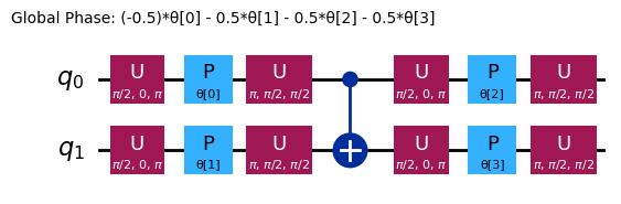
Les différents ansätze ont des structures d'enchevêtrement et des portes de rotation différentes. Celui présenté ici utilise des portes CNOT pour l'enchevêtrement, ainsi que des portes Y et des portes RZ paramétrées pour les rotations. Remarque la taille de cet espace de paramètres : cela signifie que nous devons minimiser la fonction de coût sur 4 variables (les paramètres des portes RZ). On peut mettre cela à l'échelle, mais pas indéfiniment. En exécutant un problème similaire sur 4 qubits avec les 3 répétitions par défaut de efficient_su2, on obtient 16 paramètres variationnels.

3.2 Étape 2 : Optimiser pour le matériel cible

L'ansatz a été écrit avec des portes familières, mais notre circuit doit être transpilé pour pouvoir utiliser les portes de base implémentables sur chaque ordinateur quantique. Nous sélectionnons le backend le moins occupé.

# runtime imports
from qiskit_ibm_runtime import QiskitRuntimeService, Session
from qiskit_ibm_runtime import EstimatorV2 as Estimator

# To run on hardware, select the backend with the fewest number of jobs in the queue
service = QiskitRuntimeService()
backend = service.least_busy(operational=True, simulator=False)

print(backend)

<IBMBackend('ibm_torino')>

On peut maintenant transpiler notre circuit pour ce matériel et visualiser notre ansatz transpilé.

from qiskit.transpiler.preset_passmanagers import generate_preset_pass_manager

target = backend.target
pm = generate_preset_pass_manager(target=target, optimization_level=3)

ansatz_isa = pm.run(ansatz)

ansatz_isa.draw(output="mpl", idle_wires=False, style="iqp")

Output of the previous code cell

Remarque que les portes utilisées ont changé, et que les qubits de notre circuit abstrait ont été mappés sur des qubits numérotés différemment sur l'ordinateur quantique. Nous devons mapper notre Hamiltonien de façon identique pour que nos résultats aient un sens.

hamiltonian_isa = hamiltonian.apply_layout(layout=ansatz_isa.layout)

3.3 Étape 3 : Exécuter sur le matériel cible

3.3.1 Restitution des valeurs

Nous définissons ici une fonction de coût qui prend en arguments les structures construites lors des étapes précédentes : les paramètres, l'ansatz et le Hamiltonien. Elle utilise également l'estimateur que nous n'avons pas encore défini. Nous incluons du code pour suivre l'historique de notre fonction de coût, afin de pouvoir vérifier le comportement de convergence.

def cost_func(params, ansatz, hamiltonian, estimator):
    """Return estimate of energy from estimator

    Parameters:
        params (ndarray): Array of ansatz parameters
        ansatz (QuantumCircuit): Parameterized ansatz circuit
        hamiltonian (SparsePauliOp): Operator representation of Hamiltonian
        estimator (EstimatorV2): Estimator primitive instance
        cost_history_dict: Dictionary for storing intermediate results

    Returns:
        float: Energy estimate
    """
    pub = (ansatz, [hamiltonian], [params])
    result = estimator.run(pubs=[pub]).result()
    energy = result[0].data.evs[0]

    cost_history_dict["iters"] += 1
    cost_history_dict["prev_vector"] = params
    cost_history_dict["cost_history"].append(energy)
    print(f"Iters. done: {cost_history_dict['iters']} [Current cost: {energy}]")

    return energy

cost_history_dict = {
    "prev_vector": None,
    "iters": 0,
    "cost_history": [],
}

Il est très avantageux de pouvoir choisir les valeurs initiales des paramètres en s'appuyant sur la connaissance du problème et les caractéristiques de l'état cible. Nous ne ferons aucune hypothèse de ce type et utiliserons des valeurs initiales aléatoires.

x0 = 2 * np.pi * np.random.random(num_params)

# This required 13 min, 20 s QPU time on an Eagle processor, 28 min total time.
with Session(backend=backend) as session:
    estimator = Estimator(mode=session)
    estimator.options.default_shots = 10000

    res = minimize(
        cost_func,
        x0,
        args=(ansatz_isa, hamiltonian_isa, estimator),
        method="cobyla",
        options={"maxiter": 50},
    )

Iters. done: 1 [Current cost: 0.010575798722044727]
Iters. done: 2 [Current cost: 0.004040015974440895]
Iters. done: 3 [Current cost: 0.0020213258785942503]
Iters. done: 4 [Current cost: 0.18723082446726014]
Iters. done: 5 [Current cost: -0.2746792152068885]
Iters. done: 6 [Current cost: -0.3094547651648519]
Iters. done: 7 [Current cost: -0.05281985428356641]
Iters. done: 8 [Current cost: 0.00808560303514377]
Iters. done: 9 [Current cost: -0.0014821685303514388]
Iters. done: 10 [Current cost: -0.004759824281150161]
Iters. done: 11 [Current cost: 0.09942328705995292]
Iters. done: 12 [Current cost: 0.01092366214057508]
Iters. done: 13 [Current cost: 0.05017497496069776]
Iters. done: 14 [Current cost: 0.13028868414310696]
Iters. done: 15 [Current cost: 0.013747803514376994]
Iters. done: 16 [Current cost: 0.2583072432944498]
Iters. done: 17 [Current cost: -0.14422125655131562]
Iters. done: 18 [Current cost: -0.0004950150347678081]
Iters. done: 19 [Current cost: 0.00681082268370607]
Iters. done: 20 [Current cost: -0.0023377795527156544]
Iters. done: 21 [Current cost: 0.6027665591169237]
Iters. done: 22 [Current cost: 0.00596641373801917]
Iters. done: 23 [Current cost: -0.008318769968051117]
Iters. done: 24 [Current cost: -0.00026683306709265246]
Iters. done: 25 [Current cost: -0.007648222843450479]
Iters. done: 26 [Current cost: 0.004121086261980831]
Iters. done: 27 [Current cost: -0.004075019968051117]
Iters. done: 28 [Current cost: -0.004419369009584665]
Iters. done: 29 [Current cost: 0.213185460054037]
Iters. done: 30 [Current cost: -0.06505919572162797]
Iters. done: 31 [Current cost: -0.5334241316590271]
Iters. done: 32 [Current cost: 0.00218370607028754]
Iters. done: 33 [Current cost: 0.09579352143666908]
Iters. done: 34 [Current cost: -0.009274800319488819]
Iters. done: 35 [Current cost: -0.44395141360688106]
Iters. done: 36 [Current cost: 0.011747104632587858]
Iters. done: 37 [Current cost: -0.003344149361022364]
Iters. done: 38 [Current cost: 0.19138183916486304]
Iters. done: 39 [Current cost: 0.013513931813145209]

On peut examiner les sorties brutes.

res

message: Return from COBYLA because the trust region radius reaches its lower bound.
 success: True
  status: 0
     fun: -0.5334241316590271
       x: [ 1.024e+00  6.459e+00  3.625e+00  4.007e+00]
    nfev: 39
   maxcv: 0.0

3.4 Étape 4 : Post-traiter les résultats

Si la procédure se termine correctement, les valeurs dans notre dictionnaire doivent être égales au vecteur solution et au nombre total d'évaluations de la fonction, respectivement. C'est facile à vérifier :

cost_history_dict

{'prev_vector': array([1.02397956, 6.45886604, 3.62479262, 4.00744128]),
 'iters': 39,
 'cost_history': [np.float64(0.010575798722044727),
  np.float64(0.004040015974440895),
  np.float64(0.0020213258785942503),
  np.float64(0.18723082446726014),
  np.float64(-0.2746792152068885),
  np.float64(-0.3094547651648519),
  np.float64(-0.05281985428356641),
  np.float64(0.00808560303514377),
  np.float64(-0.0014821685303514388),
  np.float64(-0.004759824281150161),
  np.float64(0.09942328705995292),
  np.float64(0.01092366214057508),
  np.float64(0.05017497496069776),
  np.float64(0.13028868414310696),
  np.float64(0.013747803514376994),
  np.float64(0.2583072432944498),
  np.float64(-0.14422125655131562),
  np.float64(-0.0004950150347678081),
  np.float64(0.00681082268370607),
  np.float64(-0.0023377795527156544),
  np.float64(0.6027665591169237),
  np.float64(0.00596641373801917),
  np.float64(-0.008318769968051117),
  np.float64(-0.00026683306709265246),
  np.float64(-0.007648222843450479),
  np.float64(0.004121086261980831),
  np.float64(-0.004075019968051117),
  np.float64(-0.004419369009584665),
  np.float64(0.213185460054037),
  np.float64(-0.06505919572162797),
  np.float64(-0.5334241316590271),
  np.float64(0.00218370607028754),
  np.float64(0.09579352143666908),
  np.float64(-0.009274800319488819),
  np.float64(-0.44395141360688106),
  np.float64(0.011747104632587858),
  np.float64(-0.003344149361022364),
  np.float64(0.19138183916486304),
  np.float64(0.013513931813145209)]}

fig, ax = plt.subplots()
x = np.linspace(0, 10, 50)

# Define the constant function
constant = -0.7029
y_constant = np.full_like(x, constant)
ax.plot(
    range(cost_history_dict["iters"]), cost_history_dict["cost_history"], label="VQE"
)
ax.set_xlabel("Iterations")
ax.set_ylabel("Cost")
ax.plot(y_constant, label="Target")
plt.legend()
plt.draw()

Output of the previous code cell

IBM Quantum propose d'autres ressources de formation liées au VQE. Si tu es prêt·e à mettre le VQE en pratique, consulte notre tutoriel : Estimation de l'énergie de l'état fondamental de la chaîne de Heisenberg avec VQE. Si tu veux plus d'informations sur la création de Hamiltoniens moléculaires, consulte cette leçon dans notre cours sur la Chimie quantique avec VQE. Si tu souhaites approfondir ta compréhension du fonctionnement des algorithmes variationnels comme le VQE, nous recommandons le cours Conception d'algorithmes variationnels.

Vérifie ta compréhension

Lis la question ci-dessous, réfléchis à ta réponse, puis clique sur le triangle pour révéler la solution.

Dans cette section, nous avons calculé l'énergie de l'état fondamental à partir d'un Hamiltonien. Si nous voulions appliquer cela pour, par exemple, déterminer la géométrie d'une molécule, comment pourrions-nous étendre cette approche ?

Réponse :

Il faudrait introduire des variables pour l'espacement inter-atomique et les angles entre les liaisons, puis les faire varier. Pour chaque variation de ces paramètres, on produirait un nouveau Hamiltonien (puisque les opérateurs décrivant l'énergie dépendent bien de la géométrie). Pour chaque Hamiltonien ainsi produit et mappé sur des qubits, il faudrait effectuer une optimisation similaire à celle réalisée ci-dessus. Parmi tous ces nombreux problèmes d'optimisation convergés, la géométrie qui produit l'énergie la plus basse serait celle adoptée par la nature. C'est bien plus complexe que ce qui a été montré ci-dessus. Un tel calcul est effectué pour la molécule la plus simple, $\text{H}_2$ , ici.

4. Les relations du VQE avec d'autres méthodes

Dans cette section, nous passerons en revue les avantages et les inconvénients de l'approche VQE originale et soulignerons ses relations avec d'autres algorithmes plus récents.

4.1 Les forces et les faiblesses du VQE

Certaines forces ont déjà été mentionnées. Elles comprennent :

Adaptation au matériel moderne : Certains algorithmes quantiques nécessitent des taux d'erreur bien plus faibles, s'approchant de la tolérance aux pannes à grande échelle. Ce n'est pas le cas du VQE ; il peut être implémenté sur les ordinateurs quantiques actuels.
Circuits peu profonds : Le VQE emploie souvent des circuits quantiques relativement peu profonds. Cela le rend moins vulnérable à l'accumulation d'erreurs de portes et le rend adapté à de nombreuses techniques d'atténuation des erreurs. Bien sûr, les circuits ne sont pas toujours peu profonds ; cela dépend de l'ansatz utilisé.
Polyvalence : Le VQE peut (en principe) être appliqué à tout problème pouvant être formulé comme un problème de valeurs propres/vecteurs propres. Il existe de nombreuses mises en garde qui rendent le VQE impraticable ou désavantageux pour certains problèmes. Certaines d'entre elles sont récapitulées ci-dessous.

Certaines faiblesses du VQE et les problèmes pour lesquels il est impraticable ont également été décrits plus haut. Ils comprennent :

Nature heuristique : Le VQE ne garantit pas la convergence vers la bonne énergie de l'état fondamental, car ses performances dépendent du choix de l'ansatz et des méthodes d'optimisation[1-2]. Si un mauvais ansatz est choisi, ne possédant pas l'enchevêtrement nécessaire pour l'état fondamental souhaité, aucun optimiseur classique ne peut atteindre cet état fondamental.
Potentiellement de nombreux paramètres : Un ansatz très expressif peut avoir tellement de paramètres que les itérations de minimisation deviennent très longues.
Coût de mesure élevé : Dans le VQE, un estimateur est utilisé pour estimer la valeur attendue de chaque terme du Hamiltonien. La plupart des Hamiltoniens d'intérêt comportent des termes qui ne peuvent pas être estimés simultanément. Cela peut rendre le VQE très gourmand en ressources pour les grands systèmes avec des Hamiltoniens complexes[1].
Effets du bruit : Lorsque l'optimiseur classique cherche un minimum, des calculs bruités peuvent le désorienter et l'éloigner du vrai minimum ou retarder sa convergence. Une solution possible consiste à exploiter les techniques de pointe en matière d'atténuation et de suppression des erreurs[2-3] d'IBM.
Plateaux stériles : Ces régions à gradients évanescents[2-3] existent même en l'absence de bruit, mais le bruit les rend plus problématiques, car la variation des valeurs attendues due au bruit peut être plus grande que la variation résultant de la mise à jour des paramètres dans ces régions stériles.

4.2 Relations avec d'autres approches

Adapt-VQE

L'algorithme ADAPT-VQE (Adaptive Derivative-Assembled Pseudo-Trotter Variational Quantum Eigensolver) est une amélioration de l'algorithme VQE original, conçue pour améliorer l'efficacité, la précision et la scalabilité des simulations quantiques, notamment en chimie quantique.

L'algorithme VQE original décrit tout au long de cette leçon utilise un ansatz prédéfini et fixe pour approcher l'état fondamental du système. Dans notre cas, nous avons utilisé efficient_su2, avec une seule répétition et des portes de rotation Y et RZ. Bien que les paramètres des portes RZ aient changé, la structure de cet ansatz et les portes utilisées n'ont pas changé.

ADAPT-VQE répond aux limitations du VQE grâce à une construction d'ansatz adaptative. Au lieu de partir d'un ansatz fixe, ADAPT-VQE construit dynamiquement l'ansatz de manière itérative. À chaque étape, il sélectionne l'opérateur d'un pool prédéfini (tel que les opérateurs d'excitation fermionique) qui présente le gradient le plus élevé par rapport à l'énergie. Cela garantit que seuls les opérateurs les plus impactants sont ajoutés, aboutissant à un ansatz compact et efficace[4-6]. Cette approche peut avoir plusieurs effets bénéfiques :

Profondeur de circuit réduite : En développant l'ansatz de façon incrémentale et en se concentrant uniquement sur les opérateurs nécessaires, ADAPT-VQE minimise les opérations de portes par rapport aux approches VQE traditionnelles[5,7].
Précision améliorée : La nature adaptative permet à ADAPT-VQE de récupérer davantage d'énergie de corrélation à chaque étape, ce qui le rend particulièrement efficace pour les systèmes fortement corrélés où le VQE traditionnel peine[8,9].
Scalabilité et robustesse au bruit : L'ansatz compact réduit l'accumulation d'erreurs de portes, diminue la charge de calcul et limite le nombre de paramètres variationnels à minimiser.

ADAPT-VQE n'est pas parfait pour autant. Dans certains cas, il peut se retrouver bloqué ou ralenti par des minima locaux, et il peut souffrir d'une sur-paramétrisation. Il peut également être assez gourmand en ressources, car il nécessite le calcul de gradients et l'optimisation des paramètres avec de nombreuses structures de portes.

Estimation de phase quantique (QPE)

La QPE est similaire dans son but au VQE, mais très différente dans son implémentation. La QPE nécessite des ordinateurs quantiques tolérants aux pannes en raison de ses circuits quantiques généralement profonds et du niveau élevé de cohérence qu'elle requiert. Une fois que la QPE pourra être implémentée, elle sera plus précise que le VQE. Une façon de décrire la différence est à travers la précision en fonction de la profondeur du circuit. La QPE atteint une précision $\epsilon$ avec des profondeurs de circuit évoluant comme $O(1/\epsilon)$ [10]. Le VQE nécessite $O(1/\epsilon^2)$ échantillons pour atteindre la même précision[10,11].

Krylov, SQD, QSCI, et autres dans ce cours

Le VQE a contribué à établir des algorithmes quantiques qui dépendent encore des ordinateurs classiques, non seulement pour faire fonctionner l'ordinateur quantique, mais aussi pour des parties substantielles de l'algorithme. Plusieurs de ces algorithmes sont au cœur du reste de ce cours. Nous donnons ici une explication succincte de quelques-uns d'entre eux, simplement pour les comparer et les contraster avec le VQE. Ils seront expliqués de façon bien plus détaillée dans les leçons suivantes.

Diagonalisation quantique de Krylov (KQD)

Les méthodes de sous-espace de Krylov sont des façons de projeter une matrice sur un sous-espace pour en réduire la dimension et la rendre plus maniable, tout en conservant les caractéristiques les plus importantes. Une astuce de cette méthode consiste à générer un sous-espace qui conserve ces caractéristiques ; il s'avère que la génération de ce sous-espace est étroitement liée à une méthode bien établie sur les ordinateurs quantiques appelée Trotterisation.

Il existe quelques variantes des méthodes de Krylov quantiques, mais l'approche générale est la suivante :

Utiliser l'ordinateur quantique pour générer un sous-espace (le sous-espace de Krylov) par Trotterisation
Projeter la matrice d'intérêt sur ce sous-espace de Krylov
Diagonaliser le nouveau Hamiltonien projeté à l'aide d'un ordinateur classique

Diagonalisation quantique par échantillonnage (SQD)

La diagonalisation quantique par échantillonnage (SQD) est liée à la méthode de Krylov en ce qu'elle tente également de réduire la dimension d'une matrice à diagonaliser tout en préservant les caractéristiques clés. SQD procède de la manière suivante :

Partir d'une estimation initiale de l'état fondamental et préparer le système dans cet état fondamental.
Utiliser le Sampler pour échantillonner les chaînes de bits qui composent cet état.
Utiliser la collection d'états de base de calcul du sampler comme sous-espace sur lequel projeter la matrice d'intérêt.
Diagonaliser la matrice projetée, plus petite, à l'aide d'un ordinateur classique.

Cela est lié au VQE en ce qu'il exploite l'informatique classique et quantique pour des composantes substantielles de l'algorithme. Ils partagent également tous deux l'exigence de préparer une bonne estimation initiale ou un bon ansatz. Mais la répartition du travail entre les ordinateurs classique et quantique dans SQD ressemble davantage à celle de la méthode de Krylov.

En fait, la méthode de Krylov et SQD ont récemment été combinées dans la méthode de diagonalisation quantique de Krylov par échantillonnage (SKQD) [12].

Interaction de configuration de sous-espace quantique

L'Interaction de configuration sélectionnée quantique (QSCI)[13] est un algorithme qui produit un état fondamental approché d'un Hamiltonien en échantillonnant une fonction d'onde d'essai pour identifier les états de base de calcul significatifs et générer un sous-espace pour une diagonalisation classique. SQD et QSCI utilisent tous deux un ordinateur quantique pour construire un sous-espace réduit. La force supplémentaire de QSCI réside dans sa préparation d'état, notamment dans le contexte des problèmes de chimie. Il exploite diverses stratégies telles que l'utilisation d'états évolués dans le temps [14] et un ensemble d'ansätze inspirés de la chimie. En se concentrant sur une préparation d'état efficace, QSCI réduit les coûts de calcul quantique pour les Hamiltoniens chimiques tout en maintenant une haute fidélité et en exploitant la robustesse au bruit des techniques d'échantillonnage d'états quantiques [15]. QSCI fournit également une technique de construction adaptative qui offre davantage d'ansätze pour un meilleur résultat.

Le flux de travail par défaut de QSCI pour les problèmes de chimie est le suivant :

Construire le Hamiltonien moléculaire à l'aide du logiciel de ton choix (comme SciPy).
Préparer un algorithme QSCI en sélectionnant un état initial approprié et un ansatz inspiré de la chimie avec un ensemble de paramètres présélectionnés.
Échantillonner les états de base significatifs et diagonaliser le Hamiltonien à l'aide d'un ordinateur classique pour obtenir l'énergie de l'état fondamental.
On utilise souvent la récupération de configuration [16] et la post-sélection par symétrie [15] comme technique de post-traitement.
En option, le flux de travail de QSCI adaptatif comporte une boucle d'optimisation supplémentaire de l'étape 2 à l'étape 3, en utilisant davantage d'ansätze avec des états initiaux aléatoires.

Vérifie ta compréhension

Lis les questions ci-dessous, réfléchis à tes réponses, puis clique sur les triangles pour révéler les solutions.

Qu'est-ce que le VQE a en commun avec toutes les autres méthodes listées ci-dessus (sauf la QPE qui n'est pas décrite en détail) ?

Réponse :

Toutes impliquent un état d'essai ou une fonction d'onde d'un certain type. Toutes fonctionnent mieux lorsque l'estimation initiale de cet état d'essai est excellente.

Une autre réponse correcte est qu'elles sont toutes plus faciles à implémenter lorsque le Hamiltonien est facile à mesurer (peut être trié en relativement peu de groupes d'opérateurs de Pauli qui commutent).

Qu'est-ce que le VQE n'a en commun avec aucune des autres méthodes listées ci-dessus ?

Réponse :

Les optimiseurs classiques. Aucune des autres méthodes n'utilise des algorithmes d'optimisation classiques pour sélectionner les paramètres variationnels.