Méthodes de compilation pour les circuits de simulation hamiltonienne
Estimation d'utilisation : moins d'une minute sur un processeur IBM Heron (REMARQUE : il s'agit d'une estimation uniquement. Ton temps d'exécution peut varier.)
Objectifs d'apprentissage
Après avoir suivi ce tutoriel, tu comprendras :
- Comment utiliser le transpileur Qiskit avec SABRE pour l'optimisation du placement et du routage
- Comment tirer parti du transpileur IA pour une optimisation avancée des circuits
- Comment utiliser le plugin Rustiq pour synthétiser des opérations
PauliEvolutionGatedans les circuits de simulation hamiltonienne - Comment évaluer et comparer les méthodes de compilation à l'aide de la profondeur à deux qubits, du nombre total de portes et du temps d'exécution
Prérequis
Nous te suggérons de te familiariser avec les sujets suivants avant de suivre ce tutoriel :
Contexte
La compilation de circuits quantiques transforme un algorithme quantique de haut niveau en un circuit physique respectant les contraintes du matériel cible. Une compilation efficace peut réduire significativement la profondeur du circuit et le nombre de portes, ce qui impacte directement la qualité des résultats sur les dispositifs quantiques à court terme.
Ce tutoriel évalue trois méthodes de compilation sur des circuits de simulation hamiltonienne construits avec PauliEvolutionGate. Ces circuits modélisent des interactions par paires entre qubits (tels que les termes , et ) et sont courants en chimie quantique, en physique de la matière condensée et en science des matériaux.
Les circuits de référence proviennent de la collection Hamlib, accessible via le dépôt Benchpress. Hamlib fournit un ensemble standardisé d'hamiltoniens représentatifs, ce qui permet de comparer les stratégies de compilation sur des charges de travail de simulation réalistes.
Vue d'ensemble des méthodes de compilation
Transpileur Qiskit avec SABRE
Le transpileur Qiskit utilise l'algorithme SABRE (SWAP-based BidiREctional heuristic search) pour optimiser le placement et le routage des circuits. SABRE se concentre sur la minimisation des portes SWAP et de leur impact sur la profondeur du circuit tout en respectant les contraintes de connectivité du matériel. C'est une méthode polyvalente qui offre un bon équilibre entre performance et temps de compilation. Pour plus de détails, voir [1]. Les avantages et l'exploration des paramètres de SABRE sont traités en profondeur dans un tutoriel séparé.
Transpileur IA
Le transpileur IA utilise l'apprentissage automatique pour prédire les stratégies de transpilation optimales en analysant les motifs de la structure des circuits et les contraintes matérielles. Il peut également appliquer la passe AIPauliNetworkSynthesis, qui cible les circuits de réseau de Pauli à l'aide d'une approche de synthèse basée sur l'apprentissage par renforcement. Pour plus d'informations, voir [2] et [3].
Plugin Rustiq
Le plugin Rustiq fournit des techniques de synthèse avancées spécifiquement pour les opérations PauliEvolutionGate, qui représentent les rotations de Pauli couramment utilisées dans les dynamiques trotterisées. Il est conçu pour produire des décompositions de circuits à faible profondeur pour les charges de travail de simulation hamiltonienne. Pour plus de détails, voir [4].
Métriques clés
Nous comparons les trois méthodes sur les métriques suivantes :
- Profondeur à deux qubits : La profondeur du circuit en comptant uniquement les portes à deux qubits. C'est souvent le facteur limitant pour la fidélité sur le matériel réel.
- Taille du circuit (nombre total de portes) : Le nombre total de portes dans le circuit transpilé.
- Temps d'exécution : Le temps réel pour la transpilation.
Prérequis
Avant de commencer ce tutoriel, assure-toi d'avoir installé les éléments suivants :
- Qiskit SDK v2.0 ou version ultérieure, avec prise en charge de la visualisation
- Qiskit Runtime v0.22 ou version ultérieure (
pip install qiskit-ibm-runtime) - Qiskit Aer (
pip install qiskit-aer) - Qiskit IBM Transpiler (
pip install qiskit-ibm-transpiler) - Mode local du transpileur IA Qiskit (
pip install qiskit_ibm_ai_local_transpiler) - Networkx (
pip install networkx)
Configuration
# Added by doQumentation — required packages for this notebook
!pip install -q matplotlib numpy qiskit qiskit-aer qiskit-ibm-runtime qiskit-ibm-transpiler requests scipy
from qiskit.circuit import QuantumCircuit
from qiskit_ibm_runtime import QiskitRuntimeService, SamplerV2
from qiskit.circuit.library import PauliEvolutionGate
from qiskit_ibm_transpiler import generate_ai_pass_manager
from qiskit.quantum_info import SparsePauliOp
from qiskit.transpiler.preset_passmanagers import generate_preset_pass_manager
from qiskit.transpiler.passes.synthesis.high_level_synthesis import HLSConfig
from qiskit_aer import AerSimulator
from qiskit_aer.noise import NoiseModel, depolarizing_error
from collections import Counter
from statistics import mean, stdev
from scipy.sparse import SparseEfficiencyWarning
import time
import warnings
import matplotlib.pyplot as plt
import matplotlib.ticker as ticker
import numpy as np
import json
import requests
import logging

# Suppress noisy loggers and warnings
logging.getLogger(
    "qiskit_ibm_transpiler.wrappers.ai_local_synthesis"
).setLevel(logging.ERROR)
warnings.filterwarnings("ignore", category=FutureWarning)
warnings.filterwarnings("ignore", category=SparseEfficiencyWarning)

seed = 42  # Seed for reproducibility
Connexion à un backend
Sélectionne un backend qui sera utilisé pour les exemples à petite et grande échelle. Le backend détermine la carte de couplage et les portes de base que le transpileur cible.
# QiskitRuntimeService.save_account(channel="ibm_quantum_platform",
# token="<YOUR-API-KEY>", overwrite=True, set_as_default=True)
service = QiskitRuntimeService(channel="ibm_quantum_platform")
backend = service.least_busy(operational=True, simulator=False)
print(f"Using backend: {backend.name}")
Using backend: ibm_pittsburgh
Définir les gestionnaires de passes
Configure les trois méthodes de compilation.
# SABRE pass manager (Qiskit default at optimization level 3)
pm_sabre = generate_preset_pass_manager(
    optimization_level=3, backend=backend, seed_transpiler=seed
)
# AI transpiler pass manager (local mode)
pm_ai = generate_ai_pass_manager(
    backend=backend, optimization_level=3, ai_optimization_level=3
)
Fetching 127 files: 0%| | 0/127 [00:00<?, ?it/s]
# Rustiq pass manager for PauliEvolutionGate synthesis
hls_config = HLSConfig(
    PauliEvolution=[
        (
            "rustiq",
            {
                "nshuffles": 400,
                "upto_phase": True,
                "fix_clifford": True,
                "preserve_order": False,
                "metric": "depth",
            },
        )
    ]
)
pm_rustiq = generate_preset_pass_manager(
    optimization_level=3,
    backend=backend,
    hls_config=hls_config,
    seed_transpiler=seed,
)
Définir les fonctions auxiliaires
La fonction suivante transpile une liste de circuits en utilisant un gestionnaire de passes donné et enregistre les métriques clés (profondeur à deux qubits, taille du circuit et temps d'exécution) pour chaque circuit.
def capture_transpilation_metrics(
    results, pass_manager, circuits, method_name
):
    """
    Transpile circuits and append one metrics record per circuit to
    ``results``.

    Args:
        results (list): List of dicts to append the metrics records to.
        pass_manager: Pass manager used for transpilation.
        circuits (list): List of quantum circuits to transpile.
        method_name (str): Name of the transpilation method.

    Returns:
        list: List of transpiled circuits.
    """
    transpiled_circuits = []

    for i, qc in enumerate(circuits):
        start_time = time.time()
        transpiled_qc = pass_manager.run(qc)
        end_time = time.time()

        # Decompose swaps for consistency across methods
        transpiled_qc = transpiled_qc.decompose(gates_to_decompose=["swap"])

        transpilation_time = end_time - start_time
        two_qubit_depth = transpiled_qc.depth(
            lambda x: x.operation.num_qubits == 2
        )
        circuit_size = transpiled_qc.size()

        results.append(
            {
                "method": method_name,
                "qc_name": qc.name,
                "qc_index": i,
                "num_qubits": qc.num_qubits,
                "two_qubit_depth": two_qubit_depth,
                "size": circuit_size,
                "runtime": transpilation_time,
            }
        )
        transpiled_circuits.append(transpiled_qc)
        print(
            f"[{method_name}] Circuit {i} ({qc.name}): "
            f"2Q depth={two_qubit_depth}, size={circuit_size}, "
            f"time={transpilation_time:.2f}s"
        )

    return transpiled_circuits
def _method_order(results):
    """Return the distinct method names in their first-seen order."""
    order = []
    for r in results:
        if r["method"] not in order:
            order.append(r["method"])
    return order

def print_summary_table(results):
    """
    Print the mean and standard deviation of each metric per compilation
    method, followed by the mean percent improvement relative to SABRE.
    """
    metrics = [
        ("two_qubit_depth", "2Q Depth"),
        ("size", "Gate Count"),
        ("runtime", "Runtime (s)"),
    ]
    methods = _method_order(results)
    by_method = {m: [r for r in results if r["method"] == m] for m in methods}
    sabre_by_index = {r["qc_index"]: r for r in by_method.get("SABRE", [])}

    col_w = 22
    name_w = max(len(m) for m in methods)
    header = f"{'Method':<{name_w}}" + "".join(
        f"  {label:>{col_w}}" for _, label in metrics
    )

    print("Mean +/- std per compilation method")
    print(header)
    print("-" * len(header))
    for method in methods:
        cells = []
        for key, _ in metrics:
            values = [r[key] for r in by_method[method]]
            std = stdev(values) if len(values) > 1 else 0.0
            cells.append(f"{mean(values):,.1f} +/- {std:,.1f}")
        print(
            f"{method:<{name_w}}" + "".join(f"  {c:>{col_w}}" for c in cells)
        )

    others = [m for m in methods if m != "SABRE"]
    if others and sabre_by_index:
        print()
        print("Mean % improvement vs SABRE (positive = better than SABRE)")
        print(header)
        print("-" * len(header))
        for method in others:
            cells = []
            for key, _ in metrics:
                pct = [
                    (sabre_by_index[r["qc_index"]][key] - r[key])
                    / sabre_by_index[r["qc_index"]][key]
                    * 100
                    for r in by_method[method]
                    if sabre_by_index.get(r["qc_index"])
                    and sabre_by_index[r["qc_index"]][key]
                ]
                if pct:
                    std = stdev(pct) if len(pct) > 1 else 0.0
                    cells.append(f"{mean(pct):+.1f}% +/- {std:.1f}%")
                else:
                    cells.append("n/a")
            print(
                f"{method:<{name_w}}"
                + "".join(f"  {c:>{col_w}}" for c in cells)
            )
def print_per_circuit_comparison(results, num_rows=5):
    """
    Print a per-metric comparison of the compilation methods for the
    first ``num_rows`` circuits (sorted by qubit count). The best
    (lowest) value for each metric is marked with an asterisk.
    """
    metrics = [
        ("two_qubit_depth", "2Q Depth"),
        ("size", "Gate Count"),
        ("runtime", "Runtime (s)"),
    ]
    methods = _method_order(results)

    by_index = {}
    for r in results:
        by_index.setdefault(r["qc_index"], {})[r["method"]] = r
    ordered = sorted(
        by_index.items(),
        key=lambda kv: (next(iter(kv[1].values()))["num_qubits"], kv[0]),
    )[:num_rows]

    for key, label in metrics:
        print(f"{label} (first {num_rows} circuits by qubit count); * = best")
        header = f"{'Idx':>3}  {'Circuit':<16} {'Q':>3}" + "".join(
            f"{m:>9}" for m in methods
        )
        print(header)
        print("-" * len(header))
        for idx, method_map in ordered:
            any_record = next(iter(method_map.values()))
            present = {
                m: method_map[m][key] for m in methods if m in method_map
            }
            best = min(present.values())
            line = (
                f"{idx:>3}  {any_record['qc_name'][:16]:<16} "
                f"{any_record['num_qubits']:>3}"
            )
            for m in methods:
                value = method_map[m][key]
                text = f"{value:.2f}" if key == "runtime" else f"{int(value)}"
                if value == best:
                    text += "*"
                line += f"{text:>9}"
            print(line)
        print()
Charger les circuits hamiltoniens depuis Hamlib
Nous chargeons un ensemble représentatif d'hamiltoniens depuis le dépôt Benchpress et construisons des circuits PauliEvolutionGate. Les circuits dont le nombre de qubits dépasse celui du backend sont supprimés, ainsi que les circuits dont la taille décomposée dépasse 1 500 portes (pour garder des temps de transpilation raisonnables).
# Obtain the Hamiltonian JSON from the benchpress repository
url = "https://raw.githubusercontent.com/Qiskit/benchpress/e7b29ef7be4cc0d70237b8fdc03edbd698908eff/benchpress/hamiltonian/hamlib/100_representative.json"
response = requests.get(url)
response.raise_for_status()
ham_records = json.loads(response.text)

# Remove circuits that are too large for the backend
ham_records = [
    h for h in ham_records if h["ham_qubits"] <= backend.num_qubits
]

# Build PauliEvolutionGate circuits
qc_ham_list = []
for h in ham_records:
    terms = h["ham_hamlib_hamiltonian_terms"]
    coeff = h["ham_hamlib_hamiltonian_coefficients"]
    num_qubits = h["ham_qubits"]
    name = h["ham_problem"]

    evo_gate = PauliEvolutionGate(SparsePauliOp(terms, coeff))
    qc = QuantumCircuit(num_qubits)
    qc.name = name
    qc.append(evo_gate, range(num_qubits))
    qc_ham_list.append(qc)

# Remove circuits whose decomposed size exceeds 1500 gates so that transpilation completes in a reasonable time frame
qc_ham_list = [qc for qc in qc_ham_list if qc.decompose().size() <= 1500]

print(f"Total Hamiltonian circuits loaded: {len(qc_ham_list)}")
print(
    f"Qubit range: {min(qc.num_qubits for qc in qc_ham_list)} to {max(qc.num_qubits for qc in qc_ham_list)}"
)
Total Hamiltonian circuits loaded: 42
Qubit range: 2 to 112
Divise les circuits en groupes à petite échelle (moins de 20 qubits) et à grande échelle (20 qubits ou plus).
qc_small = [qc for qc in qc_ham_list if qc.num_qubits < 20]
qc_large = [qc for qc in qc_ham_list if qc.num_qubits >= 20]

print(f"Small-scale circuits (<20 qubits): {len(qc_small)}")
print(f"Large-scale circuits (>=20 qubits): {len(qc_large)}")
Small-scale circuits (<20 qubits): 20
Large-scale circuits (>=20 qubits): 22
Aperçu de l'un des circuits hamiltoniens à petite échelle avant la transpilation.
# We decompose the circuit here, otherwise it would just be a PauliEvolutionGate box,
# which isn't very informative to look at!
qc_small[0].decompose().draw("mpl", fold=-1)

Exemple à petite échelle
Dans cette section, nous évaluons les trois méthodes de compilation sur des circuits hamiltoniens avec moins de 20 qubits. Ces circuits se transpilent rapidement et offrent une vue claire de la façon dont chaque méthode gère des circuits de complexité modérée.
Étape 1 : Transposer les entrées classiques en un problème quantique
Chaque hamiltonien est encodé sous la forme d'un circuit PauliEvolutionGate. Les circuits ont déjà été construits dans la section de configuration à partir des données de référence Hamlib.
Étape 2 : Optimiser le problème pour l'exécution sur matériel quantique
Nous transpilons tous les circuits à petite échelle en utilisant chacun des trois gestionnaires de passes, puis nous collectons les métriques.
results_small = []

tqc_sabre_small = capture_transpilation_metrics(
    results_small, pm_sabre, qc_small, "SABRE"
)
tqc_ai_small = capture_transpilation_metrics(
    results_small, pm_ai, qc_small, "AI"
)
tqc_rustiq_small = capture_transpilation_metrics(
    results_small, pm_rustiq, qc_small, "Rustiq"
)
[SABRE] Circuit 0 (all-vib-bh): 2Q depth=3, size=30, time=2.09s
[SABRE] Circuit 1 (all-vib-c2h): 2Q depth=18, size=111, time=0.01s
[SABRE] Circuit 2 (all-vib-o3): 2Q depth=6, size=58, time=0.00s
[SABRE] Circuit 3 (all-vib-c2h): 2Q depth=2, size=37, time=0.01s
[SABRE] Circuit 4 (graph-gnp_k-2): 2Q depth=24, size=126, time=0.01s
[SABRE] Circuit 5 (LiH): 2Q depth=66, size=285, time=0.01s
[SABRE] Circuit 6 (all-vib-fccf): 2Q depth=66, size=339, time=0.01s
[SABRE] Circuit 7 (all-vib-ch2): 2Q depth=88, size=413, time=0.01s
[SABRE] Circuit 8 (all-vib-f2): 2Q depth=180, size=1000, time=0.02s
[SABRE] Circuit 9 (all-vib-bhf2): 2Q depth=18, size=223, time=0.03s
[SABRE] Circuit 10 (graph-gnp_k-4): 2Q depth=122, size=675, time=0.02s
[SABRE] Circuit 11 (Be2): 2Q depth=343, size=1628, time=0.03s
[SABRE] Circuit 12 (all-vib-fccf): 2Q depth=14, size=134, time=0.00s
[SABRE] Circuit 13 (uf20-ham): 2Q depth=50, size=341, time=0.01s
[SABRE] Circuit 14 (TSP_Ncity-4): 2Q depth=118, size=615, time=0.01s
[SABRE] Circuit 15 (graph-complete_bipart): 2Q depth=232, size=1420, time=0.03s
[SABRE] Circuit 16 (all-vib-cyclo_propene): 2Q depth=18, size=354, time=0.93s
[SABRE] Circuit 17 (all-vib-hno): 2Q depth=6, size=174, time=0.14s
[SABRE] Circuit 18 (all-vib-fccf): 2Q depth=30, size=286, time=0.01s
[SABRE] Circuit 19 (tfim): 2Q depth=31, size=232, time=0.03s
[AI] Circuit 0 (all-vib-bh): 2Q depth=3, size=30, time=0.01s
Fetching 4 files: 0%| | 0/4 [00:00<?, ?it/s]
[AI] Circuit 1 (all-vib-c2h): 2Q depth=18, size=101, time=0.18s
[AI] Circuit 2 (all-vib-o3): 2Q depth=6, size=58, time=0.01s
[AI] Circuit 3 (all-vib-c2h): 2Q depth=2, size=37, time=0.01s
[AI] Circuit 4 (graph-gnp_k-2): 2Q depth=24, size=133, time=0.07s
[AI] Circuit 5 (LiH): 2Q depth=62, size=267, time=8.00s
[AI] Circuit 6 (all-vib-fccf): 2Q depth=65, size=300, time=0.18s
[AI] Circuit 7 (all-vib-ch2): 2Q depth=79, size=353, time=0.16s
[AI] Circuit 8 (all-vib-f2): 2Q depth=176, size=998, time=0.43s
[AI] Circuit 9 (all-vib-bhf2): 2Q depth=18, size=194, time=0.11s
[AI] Circuit 10 (graph-gnp_k-4): 2Q depth=114, size=668, time=0.18s
[AI] Circuit 11 (Be2): 2Q depth=292, size=1382, time=0.88s
[AI] Circuit 12 (all-vib-fccf): 2Q depth=14, size=134, time=0.01s
[AI] Circuit 13 (uf20-ham): 2Q depth=40, size=330, time=0.16s
[AI] Circuit 14 (TSP_Ncity-4): 2Q depth=96, size=600, time=0.29s
[AI] Circuit 15 (graph-complete_bipart): 2Q depth=231, size=1531, time=0.46s
[AI] Circuit 16 (all-vib-cyclo_propene): 2Q depth=18, size=309, time=0.25s
[AI] Circuit 17 (all-vib-hno): 2Q depth=10, size=198, time=0.15s
[AI] Circuit 18 (all-vib-fccf): 2Q depth=34, size=402, time=0.02s
[AI] Circuit 19 (tfim): 2Q depth=44, size=311, time=0.15s
[Rustiq] Circuit 0 (all-vib-bh): 2Q depth=3, size=30, time=0.01s
[Rustiq] Circuit 1 (all-vib-c2h): 2Q depth=13, size=69, time=0.00s
[Rustiq] Circuit 2 (all-vib-o3): 2Q depth=13, size=82, time=0.01s
[Rustiq] Circuit 3 (all-vib-c2h): 2Q depth=2, size=40, time=0.01s
[Rustiq] Circuit 4 (graph-gnp_k-2): 2Q depth=31, size=132, time=0.01s
[Rustiq] Circuit 5 (LiH): 2Q depth=59, size=285, time=0.01s
[Rustiq] Circuit 6 (all-vib-fccf): 2Q depth=34, size=193, time=0.00s
[Rustiq] Circuit 7 (all-vib-ch2): 2Q depth=49, size=302, time=0.01s
[Rustiq] Circuit 8 (all-vib-f2): 2Q depth=141, size=807, time=0.02s
[Rustiq] Circuit 9 (all-vib-bhf2): 2Q depth=13, size=146, time=0.02s
[Rustiq] Circuit 10 (graph-gnp_k-4): 2Q depth=129, size=683, time=0.02s
[Rustiq] Circuit 11 (Be2): 2Q depth=220, size=1101, time=0.02s
[Rustiq] Circuit 12 (all-vib-fccf): 2Q depth=53, size=333, time=0.01s
[Rustiq] Circuit 13 (uf20-ham): 2Q depth=63, size=425, time=0.01s
[Rustiq] Circuit 14 (TSP_Ncity-4): 2Q depth=123, size=767, time=0.02s
[Rustiq] Circuit 15 (graph-complete_bipart): 2Q depth=309, size=2107, time=0.05s
[Rustiq] Circuit 16 (all-vib-cyclo_propene): 2Q depth=16, size=283, time=0.32s
[Rustiq] Circuit 17 (all-vib-hno): 2Q depth=19, size=291, time=0.32s
[Rustiq] Circuit 18 (all-vib-fccf): 2Q depth=44, size=546, time=0.02s
[Rustiq] Circuit 19 (tfim): 2Q depth=24, size=416, time=0.01s
Le tableau ci-dessous résume la moyenne et l'écart type de chaque métrique pour l'ensemble des circuits à petite échelle, ainsi que le pourcentage d'amélioration par rapport à SABRE. Étant donné que les tailles de circuits varient beaucoup, l'écart type fournit un contexte important pour interpréter les moyennes.
print_summary_table(results_small)
Mean +/- std per compilation method
Method                2Q Depth              Gate Count             Runtime (s)
------------------------------------------------------------------------------
SABRE            71.8 +/- 89.6         424.1 +/- 446.0             0.2 +/- 0.5
AI               67.3 +/- 80.2         416.8 +/- 426.7             0.6 +/- 1.8
Rustiq           67.9 +/- 80.0         451.9 +/- 484.7             0.0 +/- 0.1

Mean % improvement vs SABRE (positive = better than SABRE)
Method                2Q Depth              Gate Count             Runtime (s)
------------------------------------------------------------------------------
AI             -2.1% +/- 19.8%         -0.6% +/- 14.7%   -5635.1% +/- 20725.2%
Rustiq        -25.3% +/- 85.4%        -16.3% +/- 50.4%         -7.0% +/- 60.6%
Le tableau par circuit montre comment chaque méthode se compare sur des circuits individuels. La meilleure valeur pour chaque métrique est marquée d'un astérisque. Remarque que pour les circuits les plus simples, les trois méthodes convergent souvent vers le même résultat.
print_per_circuit_comparison(results_small, num_rows=8)
2Q Depth (first 8 circuits by qubit count); * = best
Idx  Circuit            Q    SABRE       AI   Rustiq
----------------------------------------------------
  0  all-vib-bh         2       3*       3*       3*
  1  all-vib-c2h        3       18       18      13*
  2  all-vib-o3         4       6*       6*       13
  3  all-vib-c2h        4       2*       2*       2*
  4  graph-gnp_k-2      4      24*      24*       31
  5  LiH                4       66       62      59*
  6  all-vib-fccf       4       66       65      34*
  7  all-vib-ch2        4       88       79      49*

Gate Count (first 8 circuits by qubit count); * = best
Idx  Circuit            Q    SABRE       AI   Rustiq
----------------------------------------------------
  0  all-vib-bh         2      30*      30*      30*
  1  all-vib-c2h        3      111      101      69*
  2  all-vib-o3         4      58*      58*       82
  3  all-vib-c2h        4      37*      37*       40
  4  graph-gnp_k-2      4     126*      133      132
  5  LiH                4      285     267*      285
  6  all-vib-fccf       4      339      300     193*
  7  all-vib-ch2        4      413      353     302*

Runtime (s) (first 8 circuits by qubit count); * = best
Idx  Circuit            Q    SABRE       AI   Rustiq
----------------------------------------------------
  0  all-vib-bh         2     2.09     0.01    0.01*
  1  all-vib-c2h        3     0.01     0.18    0.00*
  2  all-vib-o3         4    0.00*     0.01     0.01
  3  all-vib-c2h        4     0.01     0.01    0.01*
  4  graph-gnp_k-2      4    0.01*     0.07     0.01
  5  LiH                4    0.01*     8.00     0.01
  6  all-vib-fccf       4     0.01     0.18    0.00*
  7  all-vib-ch2        4     0.01     0.16    0.01*
Visualiser les résultats
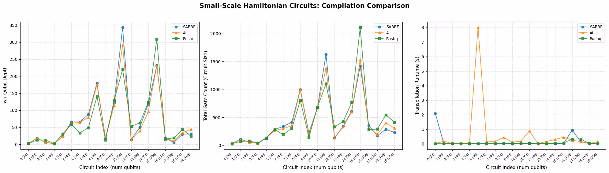
Les graphiques ci-dessous comparent les trois méthodes pour chaque métrique circuit par circuit. Les circuits sont triés par nombre de qubits et étiquetés par index sur l'axe des x, puisque plusieurs circuits peuvent avoir le même nombre de qubits.
def plot_transpilation_comparison(results, title_prefix):
    """
    Create a three-panel figure comparing compilation methods on
    two-qubit depth, circuit size, and runtime.

    Circuits are sorted by qubit count and plotted by circuit index.
    """
    methods = _method_order(results)
    palette = {"SABRE": "#1f77b4", "AI": "#ff7f0e", "Rustiq": "#2ca02c"}
    markers = {"SABRE": "o", "AI": "^", "Rustiq": "s"}

    # Order circuits by qubit count (then index) and map to plot positions
    ref = sorted(
        [r for r in results if r["method"] == methods[0]],
        key=lambda r: (r["num_qubits"], r["qc_index"]),
    )
    pos_map = {r["qc_index"]: pos for pos, r in enumerate(ref)}
    tick_positions = [pos_map[r["qc_index"]] for r in ref]
    tick_labels = [
        f"{pos_map[r['qc_index']]} ({r['num_qubits']}q)" for r in ref
    ]

    metrics = [
        ("two_qubit_depth", "Two-Qubit Depth"),
        ("size", "Total Gate Count (Circuit Size)"),
        ("runtime", "Transpilation Runtime (s)"),
    ]

    fig, axes = plt.subplots(1, 3, figsize=(20, 5.5))
    fig.suptitle(title_prefix, fontsize=15, fontweight="bold", y=1.02)

    for ax, (metric, ylabel) in zip(axes, metrics):
        for method in methods:
            subset = sorted(
                [r for r in results if r["method"] == method],
                key=lambda r: pos_map[r["qc_index"]],
            )
            ax.plot(
                [pos_map[r["qc_index"]] for r in subset],
                [r[metric] for r in subset],
                marker=markers.get(method, "o"),
                label=method,
                color=palette.get(method, None),
                linewidth=1.5,
                markersize=6,
                alpha=0.85,
            )
        ax.set_xlabel("Circuit Index (num qubits)", fontsize=11)
        ax.set_ylabel(ylabel, fontsize=11)
        ax.legend(frameon=True, fontsize=9)
        ax.grid(True, linestyle="--", alpha=0.4)
        step = max(1, len(tick_positions) // 15)
        ax.set_xticks(tick_positions[::step])
        ax.set_xticklabels(
            [tick_labels[i] for i in range(0, len(tick_labels), step)],
            fontsize=7,
            rotation=45,
            ha="right",
        )

    plt.tight_layout()
    plt.show()
def plot_pct_improvement_vs_sabre(results, title_prefix):
    """
    Plot the per-circuit percent improvement of each non-SABRE method
    relative to SABRE, for each metric. A positive value means the
    method improved on SABRE; negative means SABRE was better.
    """
    metrics = [
        ("two_qubit_depth", "2Q Depth"),
        ("size", "Gate Count"),
        ("runtime", "Runtime"),
    ]
    palette = {"AI": "#ff7f0e", "Rustiq": "#2ca02c"}
    markers = {"AI": "^", "Rustiq": "s"}

    methods = _method_order(results)
    sabre = sorted(
        [r for r in results if r["method"] == "SABRE"],
        key=lambda r: (r["num_qubits"], r["qc_index"]),
    )
    other_methods = [m for m in methods if m != "SABRE"]

    tick_positions = list(range(len(sabre)))
    tick_labels = [
        f"{i} ({sabre[i]['num_qubits']}q)" for i in range(len(sabre))
    ]

    fig, axes = plt.subplots(1, 3, figsize=(20, 5.5))
    fig.suptitle(
        f"{title_prefix}: % Improvement over SABRE",
        fontsize=15,
        fontweight="bold",
        y=1.02,
    )

    for ax, (metric, label) in zip(axes, metrics):
        ax.axhline(0, color="#1f77b4", linewidth=2, label="SABRE (baseline)")
        for method in other_methods:
            data = sorted(
                [r for r in results if r["method"] == method],
                key=lambda r: (r["num_qubits"], r["qc_index"]),
            )
            pct = [
                (sabre[i][metric] - data[i][metric]) / sabre[i][metric] * 100
                for i in range(len(sabre))
            ]
            ax.plot(
                tick_positions,
                pct,
                marker=markers.get(method, "o"),
                label=method,
                color=palette.get(method, None),
                linewidth=1.5,
                markersize=6,
                alpha=0.85,
            )
        ax.set_xlabel("Circuit Index (num qubits)", fontsize=11)
        ax.set_ylabel(f"% Improvement ({label})", fontsize=11)
        ax.legend(frameon=True, fontsize=9)
        ax.grid(True, linestyle="--", alpha=0.4)
        step = max(1, len(tick_positions) // 15)
        ax.set_xticks(tick_positions[::step])
        ax.set_xticklabels(
            [tick_labels[i] for i in range(0, len(tick_labels), step)],
            fontsize=7,
            rotation=45,
            ha="right",
        )
        ylims = ax.get_ylim()
        ax.axhspan(0, max(ylims[1], 1), alpha=0.04, color="green")
        ax.axhspan(min(ylims[0], -1), 0, alpha=0.04, color="red")

    plt.tight_layout()
    plt.show()
plot_transpilation_comparison(
    results_small,
    "Small-Scale Hamiltonian Circuits: Compilation Comparison",
)
plot_pct_improvement_vs_sabre(
    results_small,
    "Small-Scale Hamiltonian Circuits",
)
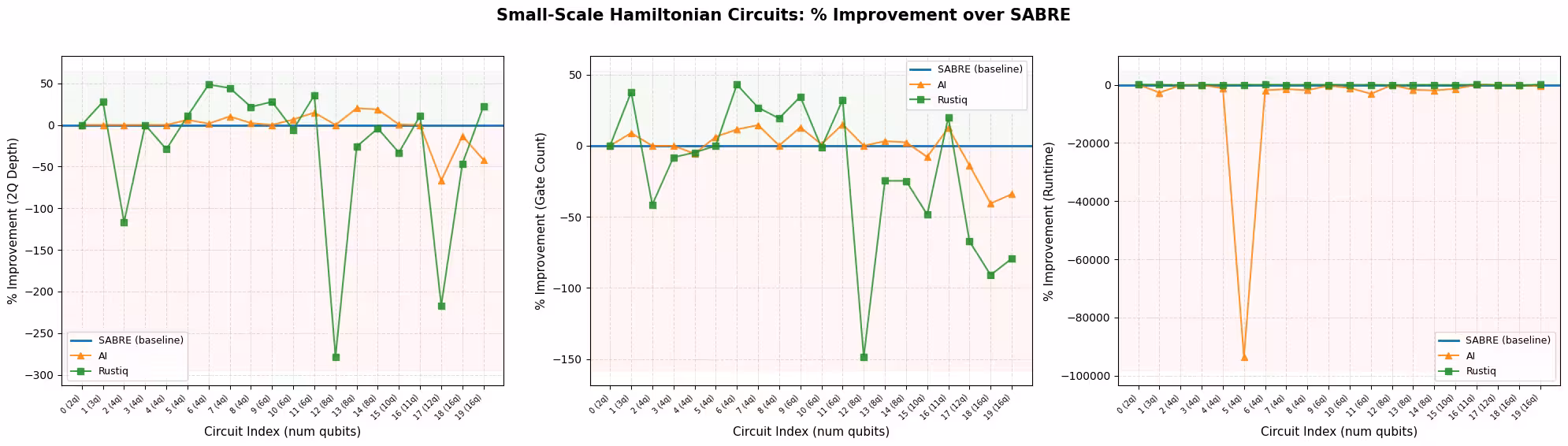
À cette échelle, les trois gestionnaires de passes donnent de bons résultats et leurs moyennes sont proches les unes des autres. Cela s'explique en grande partie parce que les petits circuits laissent peu de place à d'autres optimisations, de sorte que les méthodes tendent à converger vers des solutions similaires.
Dans cet exemple, Rustiq produit les résultats les plus variables, avec les valeurs aberrantes les plus importantes en termes de profondeur à deux qubits et de nombre de portes. Si cette variabilité signifie qu'il est parfois en retard, elle signifie aussi que Rustiq trouve parfois de meilleures solutions que les deux autres méthodes. Le transpileur IA est plus stable dans ses résultats par rapport à SABRE et Rustiq, se rapprochant étroitement de la plupart des circuits sans beaucoup de valeurs aberrantes.
Pour le temps d'exécution, SABRE et Rustiq sont tous deux rapides, tandis que le transpileur IA est notablement plus lent sur certains circuits.
Meilleure méthode par métrique
Le graphique ci-dessous montre combien de fois chaque méthode a obtenu la meilleure valeur (la plus basse) pour chaque métrique. Les égalités sont possibles : pour les circuits plus simples, plusieurs méthodes peuvent atteindre la même profondeur à deux qubits ou le même nombre de portes optimal. Lorsqu'une égalité se produit, toutes les méthodes à égalité reçoivent du crédit, de sorte que les pourcentages pour une métrique donnée peuvent totaliser plus de 100 %.
def plot_best_method_bars(results, metrics_list=None):
    """
    Plot a grouped bar chart showing the percentage of circuits
    where each method achieved the best (lowest) value for each metric.

    Ties are counted for all tied methods, so percentages per metric
    can sum to more than 100%.
    """
    if metrics_list is None:
        metrics_list = ["two_qubit_depth", "size", "runtime"]

    labels = {
        "two_qubit_depth": "2Q Depth",
        "size": "Gate Count",
        "runtime": "Runtime",
    }
    methods = _method_order(results)
    palette = {"SABRE": "#1f77b4", "AI": "#ff7f0e", "Rustiq": "#2ca02c"}

    by_index = {}
    for r in results:
        by_index.setdefault(r["qc_index"], []).append(r)
    n_circuits = len(by_index)

    win_data = {m: [] for m in methods}
    tie_counts = []
    metric_labels = []

    for metric in metrics_list:
        metric_labels.append(
            labels.get(metric, metric.replace("_", " ").title())
        )
        counts = Counter()
        ties = 0
        for group in by_index.values():
            min_val = min(r[metric] for r in group)
            best = [r["method"] for r in group if r[metric] == min_val]
            if len(best) > 1:
                ties += 1
            counts.update(best)
        tie_counts.append(ties)
        for m in methods:
            win_data[m].append(counts.get(m, 0) / n_circuits * 100)

    x = np.arange(len(metric_labels))
    width = 0.22
    fig, ax = plt.subplots(figsize=(8, 5))

    for i, method in enumerate(methods):
        bars = ax.bar(
            x + i * width,
            win_data[method],
            width,
            label=method,
            color=palette.get(method, None),
            edgecolor="black",
            linewidth=0.5,
        )
        for bar in bars:
            height = bar.get_height()
            if height > 0:
                ax.text(
                    bar.get_x() + bar.get_width() / 2,
                    height + 1.5,
                    f"{height:.0f}%",
                    ha="center",
                    va="bottom",
                    fontsize=9,
                )

    # Annotate tie counts below each metric label
    for j, ties in enumerate(tie_counts):
        if ties > 0:
            ax.text(
                x[j] + width,
                -8,
                f"({ties} tie{'s' if ties != 1 else ''})",
                ha="center",
                va="top",
                fontsize=8,
                color="gray",
            )

    ax.set_xticks(x + width)
    ax.set_xticklabels(metric_labels, fontsize=11)
    ax.set_ylabel("Circuits with best value (%)", fontsize=11)
    ax.set_title(
        "Best-Performing Method by Metric (ties counted for all tied methods)",
        fontsize=12,
        fontweight="bold",
    )
    ax.legend(frameon=True, fontsize=10)
    ax.set_ylim(-12, 120)
    ax.yaxis.set_major_formatter(ticker.PercentFormatter())
    ax.grid(axis="y", linestyle="--", alpha=0.4)

    plt.tight_layout()
    plt.show()
plot_best_method_bars(results_small)

Dans cet exemple, les trois méthodes se comportent de manière très similaire sur les circuits à petite échelle. Sur la profondeur à deux qubits et le nombre de portes, la part des circuits où chaque méthode est la meilleure est proche (environ 35–55 %), et de nombreux circuits se terminent en égalité car les circuits les plus simples ont souvent une solution optimale unique que plusieurs méthodes trouvent. La différence la plus nette est le temps d'exécution : SABRE et Rustiq sont chacun les plus rapides sur environ la moitié des circuits, tandis que le transpileur IA est rarement le plus rapide. En tenant compte des trois métriques ensemble, Rustiq présente un léger avantage global il est le plus souvent gagnant sur la profondeur à deux qubits et reste compétitif sur le nombre de portes et le temps d'exécution.
Étape 3 : Exécuter à l'aide des primitives Qiskit
Pour évaluer comment la qualité de la transpilation affecte l'exécution sous bruit, nous utilisons une technique de circuit miroir. Pour chaque circuit transpilé , nous ajoutons son inverse de sorte que le circuit combiné soit théoriquement l'identité. En partant de l'état , une exécution parfaite (sans bruit) retournerait la chaîne de bits tout-zéros avec probabilité 1.
En pratique, les erreurs de porte s'accumulent tout au long du circuit, de sorte que la probabilité de récupérer diminue. Une méthode de compilation qui produit un circuit plus superficiel avec moins de portes accumulera moins de bruit.
L'approche du circuit miroir est séduisante par sa simplicité et peut s'adapter à n'importe quelle taille de circuit, puisque la sortie attendue est toujours et qu'aucune simulation classique de l'état idéal n'est nécessaire. Cependant, note les mises en garde suivantes : le circuit miroir est un proxy pour le circuit réel (pas le circuit lui-même), il double le nombre de portes (ce qui exagère l'effet du bruit), et il peut sous-estimer certaines erreurs lorsque le bruit s'annule symétriquement à travers la frontière du miroir.
Nous sélectionnons le circuit d'index 6 dans l'ensemble à petite échelle et exécutons les circuits miroirs sur un simulateur Aer avec un modèle de bruit dépolarisant simple.
# Select circuit index 6 from the small-scale transpiled circuits
test_idx = 6
test_circuit = qc_small[test_idx]
print(f"Test circuit: {test_circuit.name}, {test_circuit.num_qubits} qubits")

# Get the transpiled versions
tqc_methods_small = {
    "SABRE": tqc_sabre_small[test_idx],
    "AI": tqc_ai_small[test_idx],
    "Rustiq": tqc_rustiq_small[test_idx],
}

# Show transpilation metrics for this circuit
print(f"\nTranspilation metrics for circuit index {test_idx}:")
for method, tqc in tqc_methods_small.items():
    depth_2q = tqc.depth(lambda x: x.operation.num_qubits == 2)
    size = tqc.size()
    print(f"  {method:8s}  2Q depth={depth_2q:5d}  size={size:6d}")
Test circuit: all-vib-fccf, 4 qubits

Transpilation metrics for circuit index 6:
  SABRE     2Q depth=   66  size=   339
  AI        2Q depth=   65  size=   300
  Rustiq    2Q depth=   34  size=   193
Construit les circuits miroirs (ajout de ), remappage vers des indices de qubits contigus afin que le simulateur ne gère que les qubits actifs, et exécution sur un simulateur Aer bruité.
def remap_to_contiguous(tqc):
    """Remap a transpiled circuit to use contiguous qubit indices.

    Transpiled circuits target specific physical qubits (e.g., qubit 45, 67)
    on a large backend. This remaps them to 0, 1, 2, ... so Aer only
    simulates the active qubits.
    """
    active = sorted(
        {tqc.find_bit(q).index for inst in tqc.data for q in inst.qubits}
    )
    qubit_map = {old: new for new, old in enumerate(active)}
    new_qc = QuantumCircuit(len(active))
    for inst in tqc.data:
        old_indices = [tqc.find_bit(q).index for q in inst.qubits]
        new_qc.append(inst.operation, [qubit_map[i] for i in old_indices])
    return new_qc

def build_mirror_circuit(tqc):
    """Build a mirror circuit: U followed by U-dagger, with measurements.

    The combined circuit U-dagger @ U should be the identity, so measuring
    all zeros indicates a noise-free execution.
    """
    tqc_compact = remap_to_contiguous(tqc)
    mirror = tqc_compact.compose(tqc_compact.inverse())
    mirror.measure_all()
    return mirror

# Build a simple depolarizing noise model
noise_model = NoiseModel()
noise_model.add_all_qubit_quantum_error(
    depolarizing_error(0.001, 1),
    ["sx", "x", "rz"],  # ~0.1% per 1Q gate
)
noise_model.add_all_qubit_quantum_error(
    depolarizing_error(0.01, 2),
    ["cx", "ecr"],  # ~1% per 2Q gate
)

aer_sim = AerSimulator(noise_model=noise_model)

shots = 10000
fidelities = {}

for method, tqc in tqc_methods_small.items():
    mirror = build_mirror_circuit(tqc)

    sampler = SamplerV2(mode=aer_sim)
    job = sampler.run([mirror], shots=shots)
    result = job.result()
    counts = result[0].data.meas.get_counts()

    # Fidelity = fraction of all-zeros (error-free) outcomes
    n_qubits = mirror.num_qubits - mirror.num_clbits  # active qubits
    all_zeros = "0" * mirror.num_qubits
    fidelity = counts.get(all_zeros, 0) / shots
    fidelities[method] = fidelity
    print(
        f"{method:8s}  P(|00...0>) = {fidelity:.4f}  ({counts.get(all_zeros, 0)}/{shots})"
    )
SABRE     P(|00...0>) = 0.7796  (7796/10000)
AI        P(|00...0>) = 0.8073  (8073/10000)
Rustiq    P(|00...0>) = 0.8923  (8923/10000)
def plot_mirror_results(tqc_methods, fidelities, circuit_name):
    """
    Plot a three-panel comparison: fidelity, 2Q depth,
    and gate count for each compilation method.
    """
    methods = list(tqc_methods.keys())
    palette = {"SABRE": "#1f77b4", "AI": "#ff7f0e", "Rustiq": "#2ca02c"}
    colors = [palette.get(m, "gray") for m in methods]

    fidelity_vals = [fidelities[m] for m in methods]
    depth_vals = [
        tqc_methods[m].depth(lambda x: x.operation.num_qubits == 2)
        for m in methods
    ]
    size_vals = [tqc_methods[m].size() for m in methods]

    fig, axes = plt.subplots(1, 3, figsize=(16, 5))
    fig.suptitle(
        f"Mirror Circuit Results: {circuit_name}",
        fontsize=14,
        fontweight="bold",
        y=1.02,
    )

    def _annotate_bars(ax, bars, values, fmt="{}"):
        ymax = ax.get_ylim()[1]
        for bar, val in zip(bars, values):
            label = fmt.format(val)
            y = val + ymax * 0.03
            ax.text(
                bar.get_x() + bar.get_width() / 2,
                y,
                label,
                ha="center",
                va="bottom",
                fontsize=10,
                fontweight="bold",
            )

    # Panel 1: Survival Probability
    bars = axes[0].bar(
        methods, fidelity_vals, color=colors, edgecolor="black", linewidth=0.5
    )
    axes[0].set_ylabel("Fidelity  P(|00...0>)", fontsize=11)
    axes[0].set_title("Fidelity (higher is better)", fontsize=12)
    axes[0].set_ylim(
        0, max(fidelity_vals) * 1.18 if max(fidelity_vals) > 0 else 1.0
    )
    axes[0].grid(axis="y", linestyle="--", alpha=0.4)
    _annotate_bars(axes[0], bars, fidelity_vals, fmt="{:.4f}")

    # Panel 2: Two-Qubit Depth
    bars = axes[1].bar(
        methods, depth_vals, color=colors, edgecolor="black", linewidth=0.5
    )
    axes[1].set_ylabel("Two-Qubit Depth", fontsize=11)
    axes[1].set_title("2Q Depth (lower is better)", fontsize=12)
    axes[1].set_ylim(0, max(depth_vals) * 1.18)
    axes[1].grid(axis="y", linestyle="--", alpha=0.4)
    _annotate_bars(axes[1], bars, depth_vals)

    # Panel 3: Gate Count
    bars = axes[2].bar(
        methods, size_vals, color=colors, edgecolor="black", linewidth=0.5
    )
    axes[2].set_ylabel("Total Gate Count", fontsize=11)
    axes[2].set_title("Gate Count (lower is better)", fontsize=12)
    axes[2].set_ylim(0, max(size_vals) * 1.18)
    axes[2].grid(axis="y", linestyle="--", alpha=0.4)
    _annotate_bars(axes[2], bars, size_vals)

    plt.tight_layout()
    plt.show()

plot_mirror_results(tqc_methods_small, fidelities, test_circuit.name)
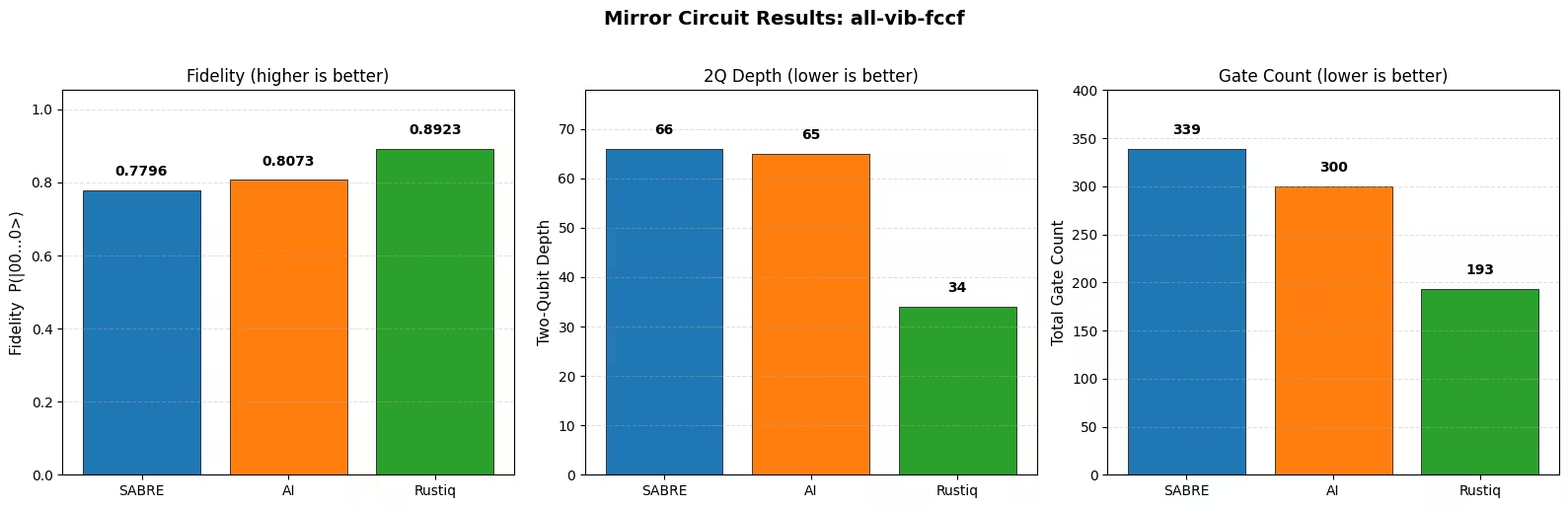
Observations
La méthode avec la profondeur à deux qubits la plus faible et le moins de portes atteint la fidélité la plus élevée, ce qui est cohérent avec l'attente que les circuits plus courts accumulent moins de bruit. Même des différences modestes de profondeur et de nombre de portes se traduisent par des différences mesurables de fidélité sous le modèle de bruit dépolarisant.
Garde à l'esprit que ces résultats concernent un seul circuit. Le classement relatif des méthodes peut changer d'un circuit à l'autre selon la structure de l'hamiltonien.
Exemple à grande échelle sur matériel
Dans cette section, nous évaluons les mêmes trois méthodes de compilation sur des circuits hamiltoniens avec 20 qubits ou plus. Ces circuits sont plus représentatifs des charges de travail pratiques de simulation hamiltonienne et testent comment chaque méthode passe à l'échelle en termes de qualité de circuit et de temps de compilation.
Étapes 1 à 4 combinées
Le flux de travail suit la même structure que l'exemple à petite échelle. Nous transpilons tous les circuits à grande échelle avec chaque méthode, collectons les métriques et soumettons un circuit miroir au matériel quantique réel.
results_large = []

tqc_sabre_large = capture_transpilation_metrics(
    results_large, pm_sabre, qc_large, "SABRE"
)
tqc_ai_large = capture_transpilation_metrics(
    results_large, pm_ai, qc_large, "AI"
)
tqc_rustiq_large = capture_transpilation_metrics(
    results_large, pm_rustiq, qc_large, "Rustiq"
)
[SABRE] Circuit 0 (all-vib-hc3h2cn): 2Q depth=2, size=258, time=0.16s
[SABRE] Circuit 1 (ham-graph-gnp_k-5): 2Q depth=345, size=4036, time=0.08s
[SABRE] Circuit 2 (TSP_Ncity-5): 2Q depth=187, size=2045, time=0.04s
[SABRE] Circuit 3 (tfim): 2Q depth=100, size=489, time=0.21s
[SABRE] Circuit 4 (all-vib-h2co): 2Q depth=30, size=570, time=0.18s
[SABRE] Circuit 5 (uuf100-ham): 2Q depth=414, size=4779, time=0.09s
[SABRE] Circuit 6 (uuf100-ham): 2Q depth=523, size=5667, time=0.11s
[SABRE] Circuit 7 (graph-gnp_k-4): 2Q depth=3028, size=24885, time=0.39s
[SABRE] Circuit 8 (uf100-ham): 2Q depth=700, size=8271, time=0.15s
[SABRE] Circuit 9 (uf100-ham): 2Q depth=698, size=8957, time=0.15s
[SABRE] Circuit 10 (TSP_Ncity-7): 2Q depth=432, size=6353, time=0.12s
[SABRE] Circuit 11 (all-vib-cyclo_propene): 2Q depth=30, size=1144, time=0.20s
[SABRE] Circuit 12 (TSP_Ncity-8): 2Q depth=704, size=10287, time=0.18s
[SABRE] Circuit 13 (uf100-ham): 2Q depth=2454, size=30195, time=0.46s
[SABRE] Circuit 14 (tfim): 2Q depth=245, size=3670, time=0.08s
[SABRE] Circuit 15 (flat100-ham): 2Q depth=154, size=3836, time=0.12s
[SABRE] Circuit 16 (graph-regular_reg-4): 2Q depth=863, size=14063, time=0.22s
[SABRE] Circuit 17 (tfim): 2Q depth=581, size=8810, time=0.15s
[SABRE] Circuit 18 (FH_D-1): 2Q depth=1704, size=9528, time=0.35s
[SABRE] Circuit 19 (TSP_Ncity-10): 2Q depth=1091, size=22041, time=0.38s
[SABRE] Circuit 20 (TSP_Ncity-10): 2Q depth=1091, size=22005, time=0.38s
[SABRE] Circuit 21 (ham-unary-color02-queen13_13_k-4): 2Q depth=224, size=8321, time=0.17s
[AI] Circuit 0 (all-vib-hc3h2cn): 2Q depth=2, size=258, time=0.17s
[AI] Circuit 1 (ham-graph-gnp_k-5): 2Q depth=323, size=4418, time=3.13s
[AI] Circuit 2 (TSP_Ncity-5): 2Q depth=161, size=2229, time=1.47s
[AI] Circuit 3 (tfim): 2Q depth=20, size=402, time=0.34s
[AI] Circuit 4 (all-vib-h2co): 2Q depth=38, size=661, time=0.19s
[AI] Circuit 5 (uuf100-ham): 2Q depth=391, size=5130, time=3.27s
[AI] Circuit 6 (uuf100-ham): 2Q depth=463, size=6095, time=4.23s
[AI] Circuit 7 (graph-gnp_k-4): 2Q depth=3207, size=25641, time=15.15s
[AI] Circuit 8 (uf100-ham): 2Q depth=637, size=8267, time=5.87s
[AI] Circuit 9 (uf100-ham): 2Q depth=632, size=9330, time=7.29s
[AI] Circuit 10 (TSP_Ncity-7): 2Q depth=452, size=7418, time=6.02s
[AI] Circuit 11 (all-vib-cyclo_propene): 2Q depth=38, size=1323, time=0.27s
[AI] Circuit 12 (TSP_Ncity-8): 2Q depth=609, size=11131, time=10.07s
[AI] Circuit 13 (uf100-ham): 2Q depth=2251, size=31128, time=38.77s
[AI] Circuit 14 (tfim): 2Q depth=165, size=3460, time=1.64s
[AI] Circuit 15 (flat100-ham): 2Q depth=91, size=3497, time=2.49s
[AI] Circuit 16 (graph-regular_reg-4): 2Q depth=664, size=15256, time=12.35s
[AI] Circuit 17 (tfim): 2Q depth=583, size=9157, time=6.28s
[AI] Circuit 18 (FH_D-1): 2Q depth=1193, size=7754, time=4.54s
[AI] Circuit 19 (TSP_Ncity-10): 2Q depth=1134, size=22577, time=25.64s
[AI] Circuit 20 (TSP_Ncity-10): 2Q depth=1172, size=23851, time=28.97s
[AI] Circuit 21 (ham-unary-color02-queen13_13_k-4): 2Q depth=219, size=8600, time=8.85s
[Rustiq] Circuit 0 (all-vib-hc3h2cn): 2Q depth=2, size=257, time=0.16s
[Rustiq] Circuit 1 (ham-graph-gnp_k-5): 2Q depth=640, size=5831, time=0.13s
[Rustiq] Circuit 2 (TSP_Ncity-5): 2Q depth=408, size=3985, time=0.08s
[Rustiq] Circuit 3 (tfim): 2Q depth=31, size=688, time=0.07s
[Rustiq] Circuit 4 (all-vib-h2co): 2Q depth=65, size=1058, time=2.91s
[Rustiq] Circuit 5 (uuf100-ham): 2Q depth=633, size=6757, time=0.14s
[Rustiq] Circuit 6 (uuf100-ham): 2Q depth=795, size=8495, time=0.17s
[Rustiq] Circuit 7 (graph-gnp_k-4): 2Q depth=13768, size=139793, time=2.92s
[Rustiq] Circuit 8 (uf100-ham): 2Q depth=1099, size=11878, time=0.25s
[Rustiq] Circuit 9 (uf100-ham): 2Q depth=911, size=11111, time=0.22s
[Rustiq] Circuit 10 (TSP_Ncity-7): 2Q depth=1183, size=13197, time=0.27s
[Rustiq] Circuit 11 (all-vib-cyclo_propene): 2Q depth=67, size=2491, time=13.56s
[Rustiq] Circuit 12 (TSP_Ncity-8): 2Q depth=1615, size=21358, time=0.48s
[Rustiq] Circuit 13 (uf100-ham): 2Q depth=2920, size=40465, time=0.91s
[Rustiq] Circuit 14 (tfim): 2Q depth=489, size=6552, time=0.15s
[Rustiq] Circuit 15 (flat100-ham): 2Q depth=378, size=5906, time=0.14s
[Rustiq] Circuit 16 (graph-regular_reg-4): 2Q depth=12163, size=168679, time=2.94s
[Rustiq] Circuit 17 (tfim): 2Q depth=1208, size=17042, time=0.36s
[Rustiq] Circuit 18 (FH_D-1): 2Q depth=1061, size=24000, time=0.47s
[Rustiq] Circuit 19 (TSP_Ncity-10): 2Q depth=2565, size=41340, time=1.38s
[Rustiq] Circuit 20 (TSP_Ncity-10): 2Q depth=2565, size=41275, time=1.38s
[Rustiq] Circuit 21 (ham-unary-color02-queen13_13_k-4): 2Q depth=808, size=17548, time=0.42s
print_summary_table(results_large)
Mean +/- std per compilation method
Method                2Q Depth              Gate Count             Runtime (s)
------------------------------------------------------------------------------
SABRE          709.1 +/- 783.8     9,100.5 +/- 8,493.1             0.2 +/- 0.1
AI             656.6 +/- 777.5     9,435.6 +/- 8,853.0            8.5 +/- 10.2
Rustiq     2,062.5 +/- 3,631.1   26,804.8 +/- 43,403.1             1.3 +/- 2.9

Mean % improvement vs SABRE (positive = better than SABRE)
Method                2Q Depth              Gate Count             Runtime (s)
------------------------------------------------------------------------------
AI             +9.6% +/- 22.8%          -3.4% +/- 9.4%    -3620.0% +/- 2405.5%
Rustiq      -154.5% +/- 273.9%      -137.1% +/- 233.2%     -527.0% +/- 1405.5%
print_per_circuit_comparison(results_large, num_rows=8)
2Q Depth (first 8 circuits by qubit count); * = best
Idx  Circuit            Q    SABRE       AI   Rustiq
----------------------------------------------------
  0  all-vib-hc3h2cn   24       2*       2*       2*
  1  ham-graph-gnp_k-  24      345     323*      640
  2  TSP_Ncity-5       25      187     161*      408
  3  tfim              26      100      20*       31
  4  all-vib-h2co      32      30*       38       65
  5  uuf100-ham        40      414     391*      633
  6  uuf100-ham        40      523     463*      795
  7  graph-gnp_k-4     40    3028*     3207    13768

Gate Count (first 8 circuits by qubit count); * = best
Idx  Circuit            Q    SABRE       AI   Rustiq
----------------------------------------------------
  0  all-vib-hc3h2cn   24      258      258     257*
  1  ham-graph-gnp_k-  24    4036*     4418     5831
  2  TSP_Ncity-5       25    2045*     2229     3985
  3  tfim              26      489     402*      688
  4  all-vib-h2co      32     570*      661     1058
  5  uuf100-ham        40    4779*     5130     6757
  6  uuf100-ham        40    5667*     6095     8495
  7  graph-gnp_k-4     40   24885*    25641   139793

Runtime (s) (first 8 circuits by qubit count); * = best
Idx  Circuit            Q    SABRE       AI   Rustiq
----------------------------------------------------
  0  all-vib-hc3h2cn   24     0.16     0.17    0.16*
  1  ham-graph-gnp_k-  24    0.08*     3.13     0.13
  2  TSP_Ncity-5       25    0.04*     1.47     0.08
  3  tfim              26     0.21     0.34    0.07*
  4  all-vib-h2co      32    0.18*     0.19     2.91
  5  uuf100-ham        40    0.09*     3.27     0.14
  6  uuf100-ham        40    0.11*     4.23     0.17
  7  graph-gnp_k-4     40    0.39*    15.15     2.92
plot_transpilation_comparison(
    results_large,
    "Large-Scale Hamiltonian Circuits: Compilation Comparison",
)
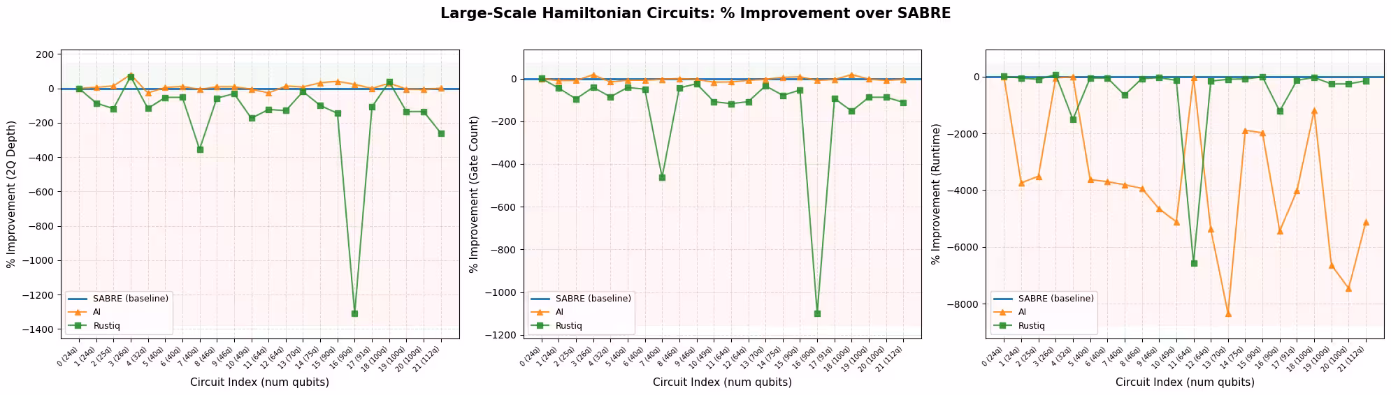
plot_pct_improvement_vs_sabre(
    results_large,
    "Large-Scale Hamiltonian Circuits",
)
plot_best_method_bars(results_large)

# Select circuit index 3 from the large-scale transpiled circuits
test_idx_large = 3
test_circuit_large = qc_large[test_idx_large]
print(
    f"Test circuit: {test_circuit_large.name}, {test_circuit_large.num_qubits} qubits"
)

tqc_methods_large = {
    "SABRE": tqc_sabre_large[test_idx_large],
    "AI": tqc_ai_large[test_idx_large],
    "Rustiq": tqc_rustiq_large[test_idx_large],
}

print(f"\nTranspilation metrics for circuit index {test_idx_large}:")
for method, tqc in tqc_methods_large.items():
    depth_2q = tqc.depth(lambda x: x.operation.num_qubits == 2)
    size = tqc.size()
    print(f"  {method:8s}  2Q depth={depth_2q:5d}  size={size:6d}")
Test circuit: tfim, 26 qubits

Transpilation metrics for circuit index 3:
  SABRE     2Q depth=  100  size=   489
  AI        2Q depth=   20  size=   402
  Rustiq    2Q depth=   31  size=   688
pm_mirror = generate_preset_pass_manager(
    optimization_level=0, backend=backend
)

for method, tqc in tqc_methods_large.items():
    # print the count ops for each circuit
    mirror = tqc.copy()
    mirror.compose(tqc.inverse(), inplace=True)
    mirror.measure_all()
    mirror = pm_mirror.run(mirror)
    print(f"\n{method} transpiled circuit:")
    print(tqc.count_ops())
    print(f"{method} mirror circuit count ops:")
    print(mirror.count_ops())
SABRE transpiled circuit:
OrderedDict({'sx': 211, 'rz': 163, 'cz': 104, 'x': 11})
SABRE mirror circuit count ops:
OrderedDict({'rz': 1170, 'sx': 422, 'cz': 208, 'measure': 156, 'x': 22, 'barrier': 1})

AI transpiled circuit:
OrderedDict({'sx': 165, 'rz': 162, 'cz': 68, 'x': 7})
AI mirror circuit count ops:
OrderedDict({'rz': 984, 'sx': 330, 'measure': 156, 'cz': 136, 'x': 14, 'barrier': 1})

Rustiq transpiled circuit:
OrderedDict({'sx': 316, 'rz': 225, 'cz': 140, 'x': 7})
Rustiq mirror circuit count ops:
OrderedDict({'rz': 1714, 'sx': 632, 'cz': 280, 'measure': 156, 'x': 14, 'barrier': 1})
# Build mirror circuits and submit to real hardware
# The inverse may introduce gates (e.g., sxdg) not in the backend's
# basis gate set, so we re-transpile the mirror circuit.
pm_mirror = generate_preset_pass_manager(
    optimization_level=0, backend=backend
)

shots_hw = 10000
hw_jobs = {}

for method, tqc in tqc_methods_large.items():
    mirror = tqc.copy()
    mirror.compose(tqc.inverse(), inplace=True)
    mirror.measure_all()

    # Re-transpile at opt level 0 to decompose into basis gates
    # without changing the layout or routing
    mirror = pm_mirror.run(mirror)

    sampler = SamplerV2(mode=backend)
    sampler.options.environment.job_tags = ["TUT_CMHSC"]
    job = sampler.run([mirror], shots=shots_hw)
    hw_jobs[method] = job
    print(f"{method}: submitted job {job.job_id()}")
SABRE: submitted job d8gvgq66983c73dqe5og
AI: submitted job d8gvgqe6983c73dqe5pg
Rustiq: submitted job d8gvgqm6983c73dqe5q0
# Retrieve results and compute fidelities
fidelities_large = {}

for method, job in hw_jobs.items():
    result = job.result()
    counts = result[0].data.meas.get_counts()

    n_qubits = backend.num_qubits
    all_zeros = "0" * n_qubits
    fidelity = counts.get(all_zeros, 0) / shots_hw
    fidelities_large[method] = fidelity
    print(
        f"{method:8s}  P(|00...0>) = {fidelity:.4f}  ({counts.get(all_zeros, 0)}/{shots_hw})"
    )
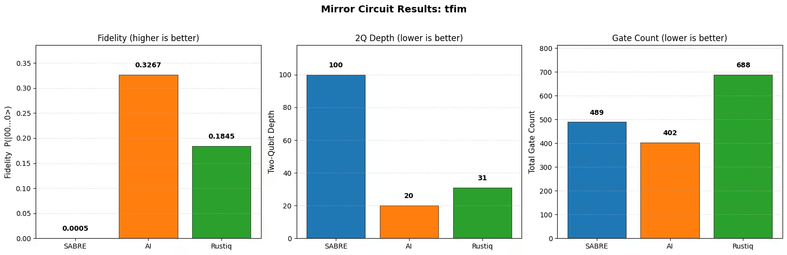
SABRE     P(|00...0>) = 0.0005  (5/10000)
AI        P(|00...0>) = 0.3267  (3267/10000)
Rustiq    P(|00...0>) = 0.1845  (1845/10000)
plot_mirror_results(
    tqc_methods_large, fidelities_large, test_circuit_large.name
)
Analyse des résultats de compilation
Les benchmarks ci-dessus comparent SABRE, le transpileur IA et Rustiq sur des circuits de simulation hamiltonienne de la collection Hamlib à petite et grande échelle.
Profondeur à deux qubits et nombre de portes
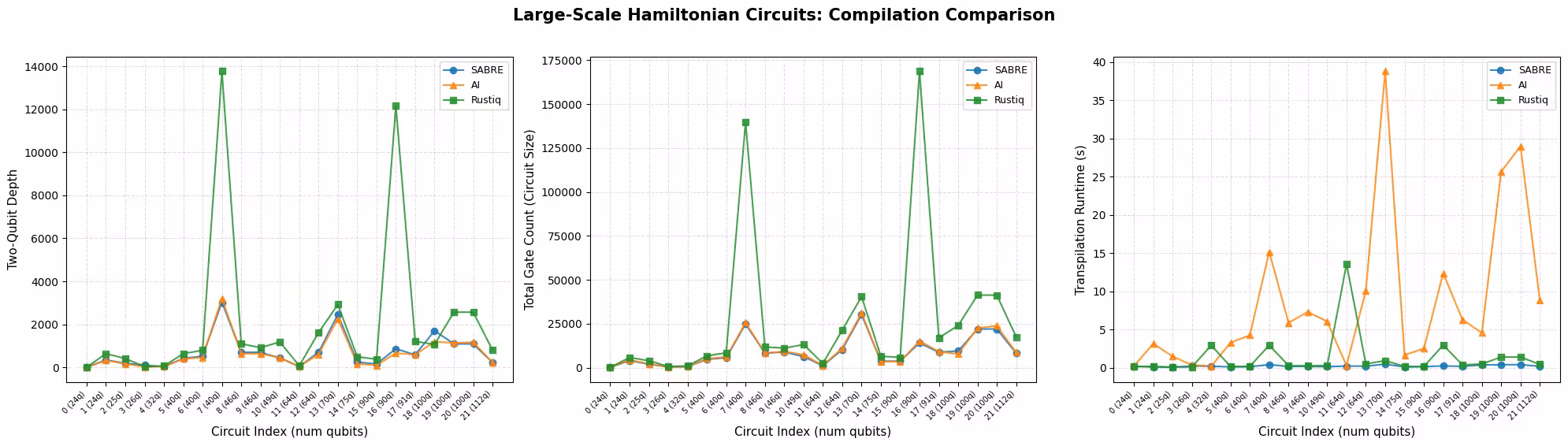
À grande échelle, SABRE et le transpileur IA sont les deux méthodes les plus performantes, et chacune mène sur une métrique différente. Comme le montre le graphique meilleure méthode par métrique, SABRE produit le nombre de portes le plus faible sur la grande majorité des circuits et est la méthode la plus rapide sur presque tous, ce qui est cohérent avec une heuristique conçue pour minimiser les portes SWAP insérées, et avec les récentes optimisations de son placement et routage. Le transpileur IA produit la profondeur à deux qubits la plus faible sur la plupart des circuits, ce qui est cohérent avec la partie de son objectif d'apprentissage par renforcement qui cible la profondeur du circuit. Le tableau récapitulatif reflète la même division : SABRE a le nombre moyen de portes le plus faible, tandis que le transpileur IA a la profondeur moyenne à deux qubits la plus faible. Les deux méthodes sont cohérentes et fiables sur l'ensemble des circuits.
Rustiq, qui est spécialement conçu pour la synthèse de PauliEvolutionGate, produit le meilleur résultat unique que sur une faible fraction des circuits à grande échelle. Ses métriques moyennes sont fortement biaisées par quelques valeurs aberrantes significatives, visibles sous forme de grands pics dans le graphique de comparaison de compilation, où Rustiq produit une profondeur et un nombre de portes substantiellement plus élevés que les autres méthodes. Sans ces valeurs aberrantes, ses performances moyennes seraient beaucoup plus proches de SABRE et du transpileur IA.
L'observation clé est qu'aucune méthode unique ne domine sur tous les circuits. Chaque méthode surpasse les autres dans des cas spécifiques, ce qui rend intéressant d'essayer tous les outils disponibles et de sélectionner le meilleur résultat pour chaque circuit.
Temps d'exécution
SABRE est systématiquement la méthode la plus rapide. Rustiq fonctionne généralement à une vitesse similaire, mais il peut produire des valeurs aberrantes où la compilation prend nettement plus de temps. Cela est particulièrement visible dans les résultats à grande échelle, où quelques circuits font augmenter le temps d'exécution de Rustiq. Ces valeurs aberrantes ont un impact important sur le temps d'exécution moyen, donc la médiane peut être un résumé plus représentatif pour Rustiq. Le transpileur IA est le plus lent des trois, avec un temps d'exécution qui augmente notablement sur des circuits plus grands et plus complexes.
Résultats du circuit miroir
Les expériences de circuit miroir confirment la tendance attendue : les méthodes qui produisent une profondeur à deux qubits plus faible et moins de portes atteignent une fidélité plus élevée sous bruit. Cela s'applique à la fois sur le simulateur bruité (petite échelle) et sur le matériel réel (grande échelle).
Garde à l'esprit que chaque graphique de circuit miroir reflète un seul circuit, pas l'agrégat. L'exemple matériel ci-dessus utilise un circuit tfim à 26 qubits, qui se trouve être un cas où SABRE produit une profondeur à deux qubits bien plus élevée que le transpileur IA et Rustiq, de sorte que sa fidélité est en conséquence beaucoup plus faible. Cela n'est pas représentatif des résultats plus larges : sur l'ensemble complet des circuits à grande échelle, la profondeur à deux qubits de SABRE est généralement proche de celle du transpileur IA, et les deux méthodes mènent chacune sur des métriques différentes (le transpileur IA sur la profondeur à deux qubits, SABRE sur le nombre de portes et le temps d'exécution). Un seul résultat miroir teste une version doublée d'un circuit plutôt que la charge de travail complète, il ne doit donc pas être lu comme un verdict sur la qualité globale de la méthode.
Recommandations
Il n'existe pas de stratégie de transpilation unique optimale pour tous les circuits. Le meilleur choix dépend de la structure du circuit, de l'objectif d'optimisation et du budget de temps de compilation disponible :
- SABRE est la valeur par défaut recommandée. Il est rapide et fiable, et produit de bons résultats sur une large gamme de circuits. Pour un réglage plus fin, les utilisateurs peuvent augmenter le nombre d'essais de placement et de routage (voir le tutoriel d'optimisation SABRE).
- Le transpileur IA vaut la peine d'être essayé lorsque le temps de compilation n'est pas une contrainte, en particulier lorsque minimiser la profondeur à deux qubits est la priorité : il a produit la profondeur à deux qubits la plus faible sur la plupart des circuits à grande échelle dans ce benchmark.
- Rustiq est spécialement conçu pour les circuits
PauliEvolutionGateet peut trouver des solutions à très faible profondeur et faible nombre de portes, en particulier sur les circuits plus petits. Sur les circuits plus grands, il peut parfois produire des résultats bien plus élevés, il est donc mieux utilisé comme l'une des plusieurs méthodes à essayer plutôt que comme choix par défaut.
En pratique, la meilleure approche est d'exécuter toutes les méthodes disponibles et de choisir le meilleur résultat pour chaque circuit. La surcharge de compilation liée à l'essai de plusieurs méthodes est faible par rapport à l'amélioration potentielle de la qualité d'exécution sur le matériel réel.
Étapes suivantes
Si tu as trouvé ce tutoriel utile, tu pourrais être intéressé par les éléments suivants :
Références
[1] "LightSABRE: A Lightweight and Enhanced SABRE Algorithm". H. Zou, M. Treinish, K. Hartman, A. Ivrii, J. Lishman et al. https://arxiv.org/abs/2409.08368
[2] "Practical and efficient quantum circuit synthesis and transpiling with Reinforcement Learning". D. Kremer, V. Villar, H. Paik, I. Duran, I. Faro, J. Cruz-Benito et al. https://arxiv.org/abs/2405.13196
[3] "Pauli Network Circuit Synthesis with Reinforcement Learning". A. Dubal, D. Kremer, S. Martiel, V. Villar, D. Wang, J. Cruz-Benito et al. https://arxiv.org/abs/2503.14448
[4] "Faster and shorter synthesis of Hamiltonian simulation circuits". T. Goubault de Brugiere, S. Martiel et al. https://arxiv.org/abs/2404.03280